7. Hydraulic fracturing

This chapter reviews the initiation and growth of fluid-driven fractures, commonly known in practice as “hydraulic fractures”. The propagation of fluid-driven fractures depends on the properties of the porous medium where the fracture propagates, the properties of the injected fluid, and the in-situ stresses. Hydraulic fractures tend to open up as planes perpendicular to the minimum principal stress in order to minimize required work to open. Open-mode fluid-driven fractures happen naturally in the subsurface, may occur accidentally during wellbore drilling, and help improve reservoir connectivity to the wellbore when used for completion purposes.

7.1 Fluid-driven fractures in nature

Hydraulic fractures are common in the subsurface and occur naturally when a fluidized material overcomes the list principal stress and required fracture propagation energy. “Fluidized materials” include typical pore fluids such as water, gases and hydrocarbons and also magma and fluidized muds. Naturally occuring hydraulic fractures with fluids may not remain open or propped and are difficult to identify in nature unless mineral precipitation makes them evident.

Magmatic dykes/dikes form when pressurized magma overcomes the minimum principal stress in the subsurface. Dykes form large vertical planes in places with marked stress anisotropy with $S_3 = S_{hmin}$. Figure 7.1 shows examples of dykes as observed on surface and in mines. Magmatic dykes tend to be easy to identify near surface because magma hardens in place and igneous rocks are hard to weather with time. In fact, magmatic dykes occur frequently near divergent boundaries and zones with thin crust. 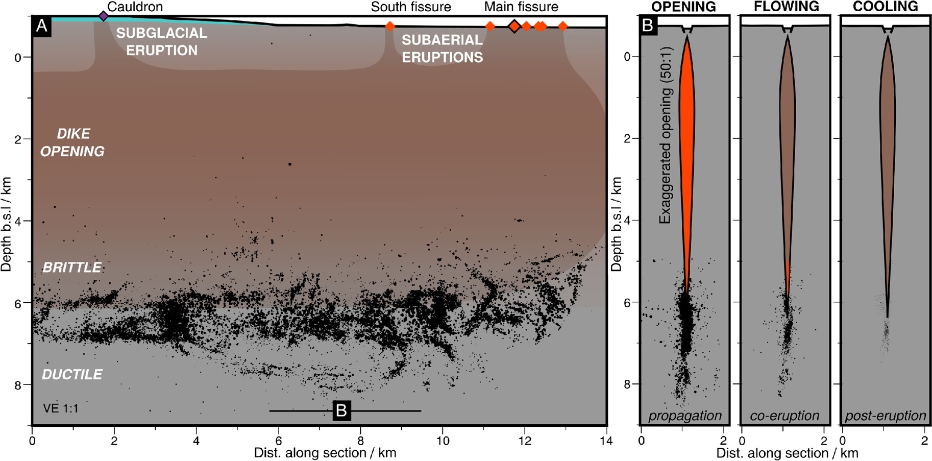Recently, dykes have been monitored through seismic activity in Iceland (Figure 7.2): the monitored horizontal propagation velocity was about 200 m/hr. Igneous dykes can cut through oil and gas basins, and regions target of carbon dioxide and hydrogen storage. 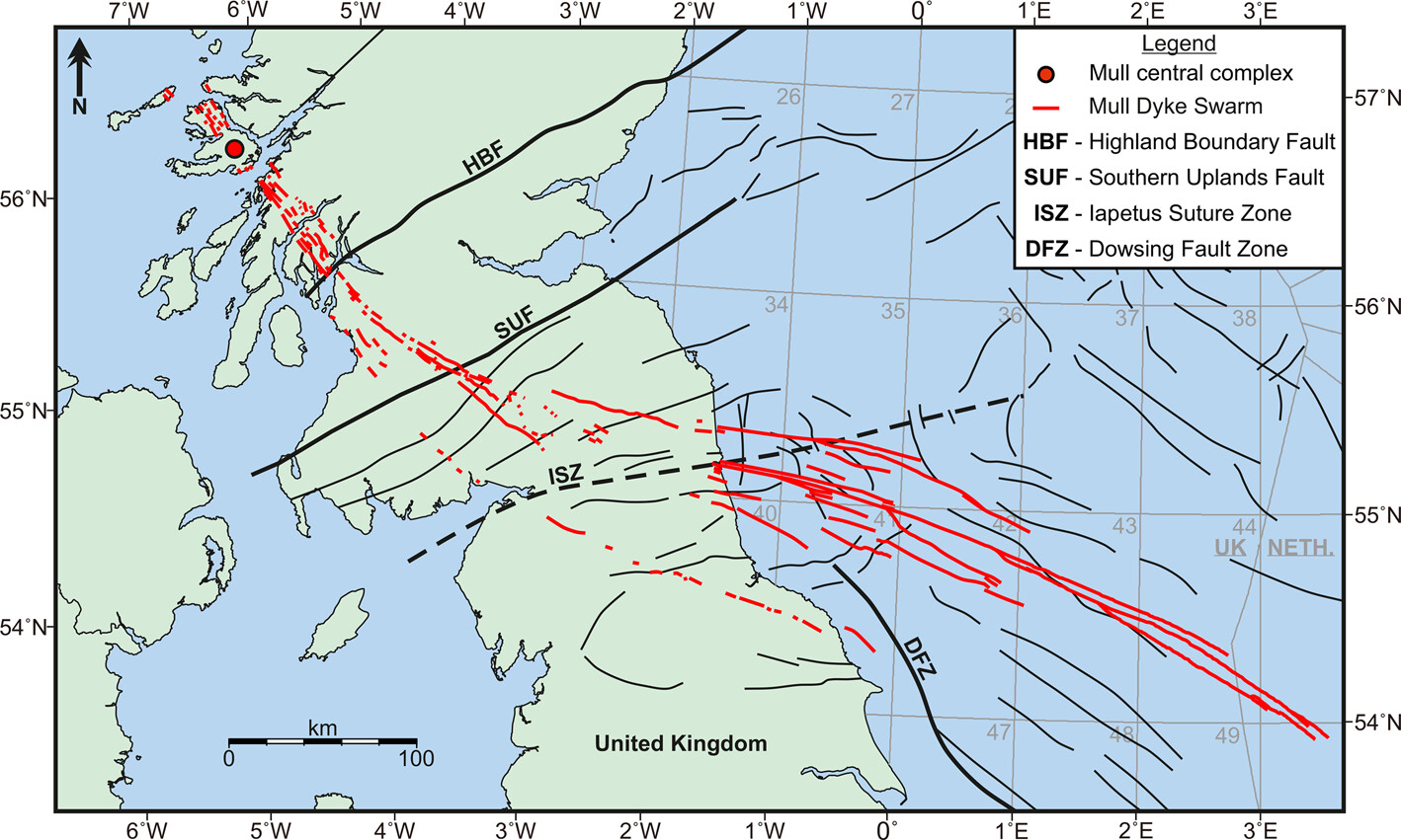Figure 7.3 shows an example of a map of dyke swarms in the North Sea. Some of these dykes are hundreds-of-kilometers long and act as seals for natural accumulations of oil and gas in the North Sea.

Figure 7.1: Formation of dykes and examples. Dykes are large and natural fluid-driven fractures.

Figure 7.2: Example of dyke propagation and monitoring through induced microseismicity (Image credit: https://doi.org/10.1016/j.epsl.2018.10.032). An animation video of the dyke propagation is available here: https://ars.els-cdn.com/content/image/1-s2.0-S0012821X18306289-mmc5.mp4.

Figure 7.3: Recent improved mapping of the Mull Dyke swarm in the UK. 100-km long dykes cross through sedimentary basins with great economic value (Image credit: https://doi.org/10.1144/jgs2023-039).

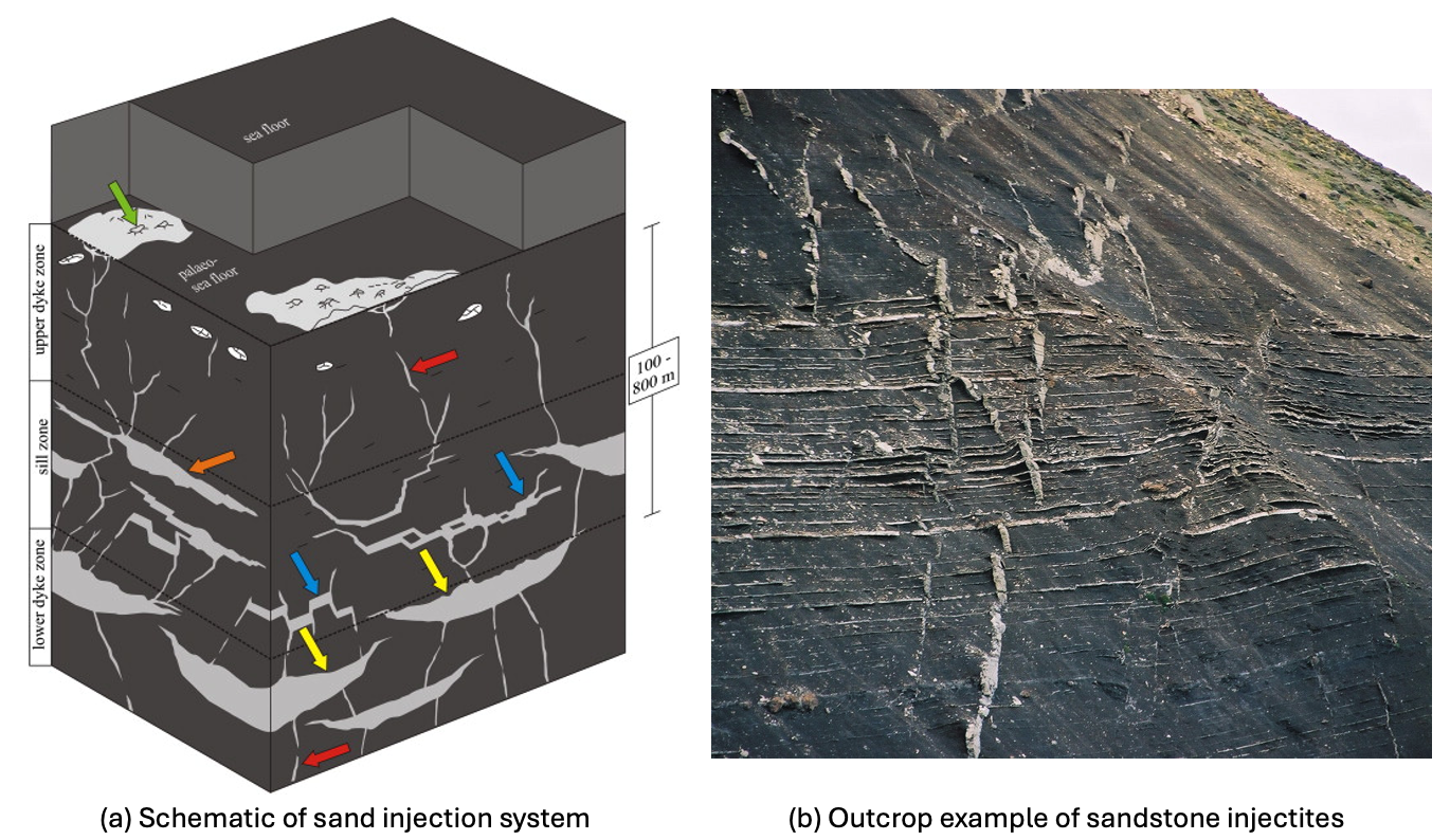
Sedimentary dykes and pipes occur when fluidized sediments create fluid driven fractures or conduits. Fluidization happens when water/gas pressure is so high that effective stress goes to zero and the sediment loses frictional strength. These sediment intrusions into upper strata are usually termed injectites when planar or mud volcanoes when predominantly one-dimensional. Figure 7.4 shows an example of interpreted sediment injectites cutting through low permeability formations and an example from the field.

Figure 7.4: Sand injectites schematic (a, image credit: https://doi.org/10.1016/j.earscirev.2011.02.004) and outcrop example in Patagonia (b, image credit: https://www.wired.com/2010/01/friday-field-foto-100-sandstone-injectites-in-patagonia/), sand horizontal thickness is about 10cm.

7.2 Hydraulic fracture injection/shut-in tests

Understanding of hydraulic fractures is important for several applications in petroleum and geosystems engineering, from drilling and completion to enhanced oil recovery. The following field tests involve hydraulic fracturing and are suitable for specific applications.

7.2.1 Leak-off test

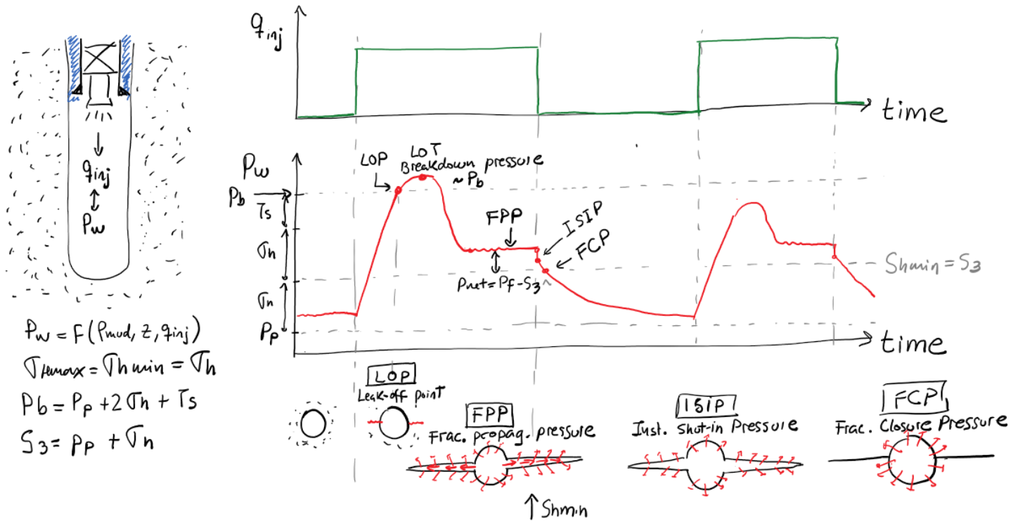
The leak-off test is conducted to measure the fracture gradient required for setting maximum mud pressure for drilling. The test is conducted with drilling mud after cementing the casing of the previous section in an open-hole.

Figure 7.5: Ideal leak off test pressure response with $S_v > S_{Hmax} = S_{hmin}$.

Execution of the leak-off test involves the following events:

• Injection of drilling mud at a constant rate causes the pressure to increase up to a maximum that depends on the near-wellbore stresses and tensile strength of the rock (Fracture breakdown pressure FBP or $P_b$). A change of slope may occur before FBP indicating a change of cavity volume, known as leak-off point (LOP).
• After fracture initiation, the fracture propagates at a velocity dictated by the fluid injection rate at a characteristic fracture propagation pressure (FPP).
• Shut-in of the pumps causes the pressure to decrease quickly at the instantaneous shut-in pressure (ISIP). Further pressure decrease originates from fluid in the fracture leaking off to the rock until the fractures closes at the fracture closure pressure (FCP).

Figure 7.6 shows an example of a leak-off test using another notation for the leak-off point and breakdown pressure. Some studies suggest that a deviation from linearity at the beggining of the test indicates the opening of a small fracture (FIP) until it reaches a maximum pressure (UFP) after which it propagates at a rate faster than the injected fluid. An “extended” leak-off test requires to reach the UFP (or FPP) pressure. Sometimes the leak-off tests may be stopped before UFP to avoid large fractures in the well.

Figure 7.6: Example of real leak-off test data from an off-shore well. The pressure data show surface pressure readings.

7.2.1.1 Determination of the instantaneous shut-in pressure (ISIP)

The shut-in pressure is the maximum pressure before the pressure signature exhibits a gradual decay as a function of time due to shutting the pumps.

Figure 7.7: Example of determination of the instantaneous shut-in pressure from a fracture test.

7.2.1.2 Determination of the fracture closure pressure (FCP)

While the fracture is still open in an uncased borehole, fluids in the fracture leak off from both the wellbore and the fracture. Large leak-off surface (fracture walls and well) causes a rapid pressure decrease approximately proportional to the $\sqrt {t_{si}}$ (where $t_{si}$ is the time after shut-in). The pressure decrease rate slows down once the fracture closes (leak-off just from well) and departs from the $P$ vs. $\sqrt {t_{si}}$ linear trend. The fracture closure pressure (FCP) is the pressure at which this change in leak-off regime occurs (See example in Fig. 7.8). Fracture closure is interpreted to be approximately equal to the minimum principal total stress $S_3$.

Figure 7.8: Example of determination of the fracture closure pressure. Departure from the linear trend in a $P$ vs. $\sqrt {t_{si}}$ plot indicates fracture closure.

7.2.2 Diagnostic fracture initiation test (DFIT)

The objectives of the DFIT test are to determine permeability, determine pore pressure, and determine minimum principal stress $S_3$. The DFIT test is usually done in tight low-permeability reservoirs for completion purposes before a large hydraulic fracture treatment. The test involves small wellbore intervals using relatively small fracturing fluid injection volumes $\leqslant 10$ bbl. The injection rates are also relatively small ranging from $\sim$0.1 to 3 bbl/min. The DFIT test may be performed through perforations in already cased boreholes.

Figure 7.9: The DFIT test is performed with small injection volumes before actual hydraulic fracture completion.

The mechanics of the DFIT test is similar to the one of the leak-off test. The determination of FCP is similar to that of the leak-off test. More advanced methods use a “G-function” to determine FCP. The G-function is a dimensionless time function designed to linearize the pressure signal during normal fluid leak-off from a bi-wing fracture.

Figure 7.10: DFIT tests often utilize a “G-function” to determine the closure pressure. This method is based on the analysis of leak-off similar to the square-root-of-time method.

7.2.3 Step-rate test

The step rate test helps determine the maximum injection pressure in a wellbore designed for constant and long-term injection. Examples of injected fluids include water (liquid or vapor), CO$_2$, N$_2$, polymer mixtures, foam, natural gas, and produced water, among others. The objective is to determine the maximum injection pressure known as “formation parting pressure”.

The Procedure of the step-rate test is the following (See Figure 7.11):

1. Isolate the injection zone.
2. Inject fluid at successively higher injection rates during equal periods of time. Suggested schedule:
   • STEP TIME: 60 min if k$<$5md and 15-30 min if k$>$10 md
   • INJECTION RATE: 5, 10, 20, 40, 60, 80, 100% of maximum expected injection rate
3. Plot maximum stabilized pressure $P$ for each step as a function of injection rate $q$
4. The formation parting pressure is identified by the change in slope of $P$ vs. $q$

Figure 7.11: Schematic procedure of an ideal step-rate test. FPR: fracture propagation rate. FPP: fracture propagation pressure. Modified from [SPE 169513]

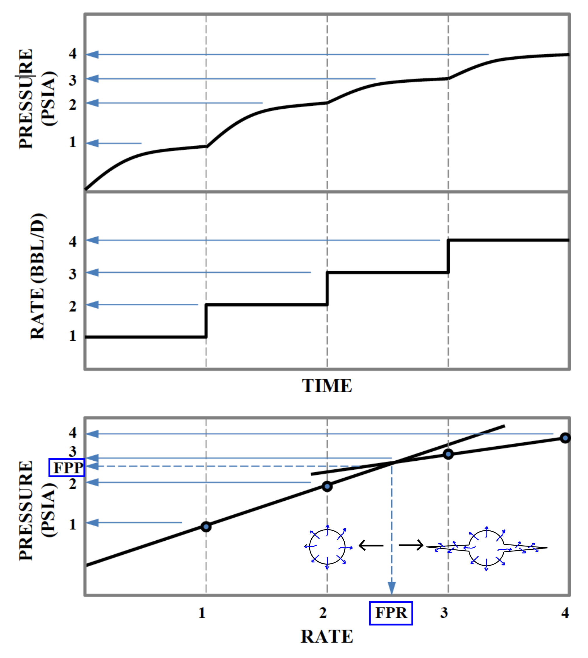Each injection step is performed until the pressure signal approaches an asymptotic response (top and middle figures). This maximum pressure $P$ at each step is then plotted as a function of injection rate $q$. The change in slope in the $P$ vs. $q$ plot (bottom) determines the formation parting pressure (FPP) and the formation parting rate (FPR). The change of slope occurs due to fracturing of the injector and can be interpreted as a change of the skin factor $s$ ($s>1$ means damage and $s<1$ means stimulation) in the wellbore equation

$$q = \frac{2 \pi h k} {\mu} \frac{P_e - P_w}{\ln (\frac{r_e}{r_w})+s}$$ (7.1)

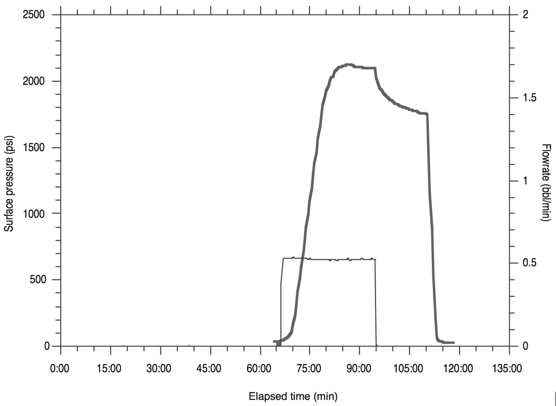
Figure 7.12 shows an example of a step rate test conducted with steam. The step-rate test is required test by some regulatory agencies in order to safely dispose produced water. The objective is to avoid fracturing of the injector. There are ongoing efforts to regulate injection of large volumes that may not fracture the injector but could reactivate neighboring faults.

Figure 7.12: Example of actual injection-rate test for steam injection in an off-shore reservoir in California [data from SPE 169513].

Unintentional fracturing of the injector can be detrimental to sweep efficiency in EOR and IOR processes if the fracture connects the injectors and producers. On the other hand, fractures can be beneficial for sweep efficiency if oriented perpendicular to the direction of sweep (Fig. 7.13).

Figure 7.13: Example of fracturing in water-flooding with detrimental (left) and beneficial (right) implications for sweep efficiency. Circle plus arrow : injector, circle: producer, HF: hydraulic fracture.

7.3 Hydraulic fracture design: Single fracture completion

7.3.1 Improvement of reservoir access and wellbore-reservoir surface area

The creation of a hydraulic fracture improves dramatically the surface area of the wellbore in contact with the formation, and also the corresponding production rates (at the same bottomhole pressure). The ratio between the area of a fracture (constant height $h$ and half-length $x_f$) and the area of an openhole wellbore (radius $r$ and height $h$) is $(4 x_f h)/(2\pi r_w h) \sim x_f/r_w$. Fractures are usually much longer than the radius of the wellbore and so does the fracture area in contact with the reservoir rock compared to the area of the wellbore. The use of a skin factor $s$ permits calculating the flow rates in the presence of the fracture using the wellbore equation (Figure 7.14).

Figure 7.14: Reservoir drainage: A fractured wellbore dramatically increases flow rates for the same bottomhole pressure. The rate is proportional to $x_f/r_w$.

7.3.2 The coupled fluid-driven fracture propagation problem

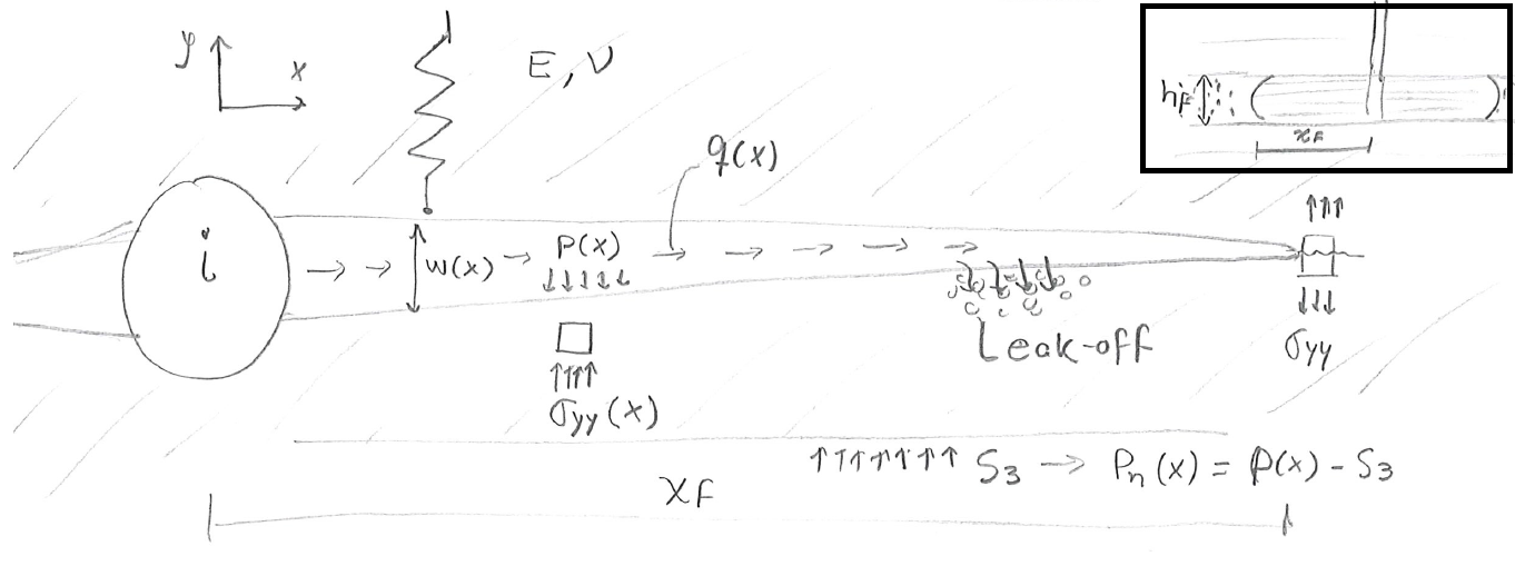
Several physical processes interact during the propagation of fluid-driven fractures (Figure 7.16). The main processes include:

1. Opening of the fracture by deformation of adjacent rock. The calculation of fracture width can be achieved by solving fracture opening, for example by solving a linear elasticity problem.
2. Creation of new fracture surface. Cemented rocks require tensile stresses at the tip surpass a certain limit in order to create new fracture surface. This problem is most times solved with the theory of linear elastic fracture mechanics.
3. Leak-off of fracturing fluid into the formation. Fracturing of porous media involves fluid flow into the fractured formation. Leak-off can be solved as any fluid flow problem or through simplified equations. Leak-off also affects effective stresses around the fracture face and tip.
4. Fluid flow within the fracture. Fracture propagation requires constant inflow of fluid into the fracture. Fluid-driven fractures in stiff rocks tend to be narrow (few millimeters) and therefore non-negligible viscous losses occur when fluids flow through fractures. This problem can be solved as a lubrication problem of fluid flow within planar surfaces.

The following subsections describe each of these problems in more detail.

Figure 7.15: The four coupled processes in fluid-driven fracture propagation in porous media.

Figure 7.16: The four coupled processes in fluid-driven fracture propagation in porous media.

7.3.2.1 Mechanics: The pressurized linear crack problem

The first step consists on solving the deformation of a fracture subjected to external far-field stresses $\uuline{S}$ and pressure in the fracture $p$. The example in Figure 7.17 shows a 2D example of a fracture within a infinitely large and impervious medium. The fracture has a fluid pressure that varies along the length of the fracture. The center is pressurized at pressure $p$ and the ends have zero pressure. The medium has a far-field minimum principal stress $S_3$ acting perpendicular to the fracture. The net pressure $p_{net}$ is defined as the difference between the fluid pressure in the fracture $p$ and least principal total stress $S_3$.

$$p_{net} = p - S_3$$ (7.2)

For example, the fracture in Figure 7.17 has positive net pressure in the center and negative net pressure in the ends. A fluid-driven fracture will open if and only if $p_{net}>0$, i.e., $p > S_3$. Also, the net pressure concept facilitates the development of analytical solutions, by combining two actions into one.

Figure 7.17: Example of the net pressure concept.

The second step is to solve the displacements and strains that occur due to pressuring a fracture with a given net pressure. This problem was solved by A. A. Griffith (https://en.wikipedia.org/wiki/Fracture_mechanics), and is known as the Griffith crack problem. Griffith assumed a homogeneous and isotropic solid to solve stresses around a fracture.

The simplest solution is the one in which the net pressure is constant along the fracture $p_{net} = p_o$. Hence, for a fracture with half-length $c$ (Fig. 7.18), the boundary conditions of the problem are:

$$\left\lbrace \begin{array}{rcl c l} \sigma_{yy} & = & p(x)= p... ...c \\ u_y & = & 0 & \text{ for } & x > c \\ \end{array}\right.$$ (7.3)

Figure 7.18: Griffith's crack problem: Geometry and assumptions of pressurized line crack in 2D elastic, isotropic, homogeneous solid.

The solution of the Navier's equation (Eq. 3.40) yields the following values at the line $(x,y=0)$:

$$\left\lbrace \begin{array}{rcl c l} u_y(x,0) & = & \cfrac{2 p... ...2-c^2}} -1 \right) & \text{ for } & x >c \\ \end{array}\right.$$ (7.4)

where $E'= E / (1 - \nu^2)$ is the plane strain modulus. Let us investigate this solution at $x=0$ and $x=c$. The displacement at $x=0$ is $u_y(0,0) = 2 p_0 c /E'$, hence, the maximum width of the fracture is

$$w_o = \frac{4 p_0 c}{E'}$$ (7.5)

It makes sense that the width of the fracture will be proportional to the net pressure and the half-length, and inversely proportional to the stiffness of the medium. The solution of $u_y$ is an elliptical equation, thus, Griffith predicts an elliptically shaped fracture when the net pressure is constant.

Let us now solve the stress at the tip of the fracture $x=c$: $\sigma_{yy}(c,0) \rightarrow - \infty$ which in practice is impossible. We will find a solution for this problem in the next subsection. The stress beyond the tip is tensile. For example at $x=1.15c$, $\sigma_{yy}(1.15c,0) \sim - p_o$.

7.3.2.2 Mechanics: stress intensity factor and fracture toughness

The previous subsection shows that the solution of stresses at the the fracture tip yields an infinitely large tensile stress. Thus, we would not be able to use the tensile strength criterion because the stress would be always larger than the theoretical stress. In order to circumvent this problem, Griffith defined the stress intensity factor as

$$K_I = \lim_{r \rightarrow 0^+} \left[ (2 \pi r)^{1/2} \sigma_{yy} (x=c+r,y=0) \right]$$ (7.6)

where $r=x-c$ is the distance from a point in the solid to the fracture tip. The solution of the stress intensity factor equation for a line crack pressurized with constant pressure $p_o$ can be obtained plugging the solution for $\sigma_{yy}$ (Eq. 7.4) and is equal to

$$K_I = p_o ( \pi c)^{1/2}$$ (7.7)

The Griffith criterion establishes that a fracture may propagate if the stress intensity $K_I$ is larger than the fracture toughness $K_{IC}$, where $K_{IC}$ is a property of the material.

$$\left\lbrace \begin{array}{rcl} K_I \geq K_{IC} & \rightarrow... ...ow & \text{ Fracture does not propagate} \\ \end{array}\right.$$ (7.8)

The superscript $I$ means that this is “Mode I” fracture, also known as opening-mode fracture. There are two other modes of fracture intensity and propagation related to in-plane shear (Mode II) and out-of-plane shear (Mode III) (Figure 4.22).

The fracture toughness $K_{IC}$ is the property of a solid and can be measured with the semicircular bending test (Fig. 7.19). Linear elasticity permits calculating the stress intensity factor, such that, the fracture toughness is

$$K_{IC} = \frac{ P_{max} ( \pi a)^{1/2} }{2rL} Y_I$$ (7.9)

where $P_{max}$ [N] is the maximum load at failure and $a$ [m] is the length of the notch pre-carved in the sample (other geometrical values in figure). The parameter $Y_I$ [-] is geometrical factor and depends on $s/r$ and it is $Y_I \sim 4.5$ for $s/r = 0.8$ and $0.1 < a/r <0.2$. Typical rock fracture toughness values vary between $K_{IC} \sim 0.05$ to 1.5 MPa m$^{1/2}$.

Figure 7.19: Geometry and variables for the semicircular bending test. The notch simulates a pre-existing fracture and intensifies stresses at the tip.

PROBLEM 7.1: Calculate the maximum width and stress intensity of a fracture with half-length $x_f = 10$ m and pressurized to $p_f = 20.5$ MPa, immersed within a elastic medium with $E = 1$ GPa and $\nu =$ 0.25, and subjected to far field stress $S_3 = 20$ MPa.

SOLUTION

Let us first compute the plane strain modulus

$$E' = \frac{E}{1-\nu^2} = \frac{1 \text{ GPa}}{1-0.25^2} = 1.07 \text{ GPa} = 1070 \text{ MPa}$$

Using Eqs. 7.7 and 7.5, and noting that the net pressure is $p_{net} = p_f - S_3$ the results are:

$$w_o = \frac{4 p_0 c}{E'} = \frac{4 \times 0.5 \text{ MPa} \times 10 \text{ m}} {1070 \text{ MPa}} = 0.019 \text{ m} = 19 \text{ mm}$$

$$K_I = p_o ( \pi c)^{1/2} = 0.5 ( \pi \times 10 )^{1/2} = 2.8 ^{1/2}$$

Extra: The assumption of constant net pressure along the fracture is not accurate for a propagating fracture. The width and stress intensity for net pressure distribution starting at $p_o$ in the center and decreasing linearly to zero at the tips are:

$$w_o = \frac{2 p_0 c}{E'} = \frac{2 \times 0.5 \text{ MPa} \times 10 \text{ m}} {1070 \text{ MPa}} = 0.0095 \text{ m} = 9.5 \text{ mm}$$

$$K_I = \left( 1-\frac{2}{\pi} \right) p_o ( \pi c)^{1/2} = \left( 1-\frac{2}{\pi} \right) 0.5 ( \pi \times 10 )^{1/2} = 1.0 ^{1/2} \: \: \blacksquare$$

7.3.2.3 Transport: leak-off

The total injected fluid $V_i$ during fracturing goes into filling the open fracture $V$ and some leaks into the formation $V_L$. Hence, material balance dictates

$$V_i = V + V_L$$ (7.10)

The leak-off volume can be calculated as a function of time $t$ as a problem of fluid flow in porous media and approximated with the Carter leak-off equation:

$$V_L = A_L (2 c_L \sqrt{t} + S_p)$$ (7.11)

where $A_L$ is the area of leak-off, $c_L$ is the Carter leak off coefficient, and $S_p$ is the instantaneous fluid spurt loss. The efficiency of injection is defined through coefficient

$$\eta = \frac{V}{V_i}$$ (7.12)

Thus, $\eta \rightarrow 1$ indicates high efficiency of the use of fracturing fluid to propagate a fracture and $\eta \rightarrow 0$ indicates significant leak-off.

The amount of injected fluid for a constant injection rate $i$ is

$$V_i = i \: t$$ (7.13)

Both $V_i$ and $i$ are defined for one-wing of the fracture. Hence, the total injected fluid through the wellbore in a bi-wing fracture is $2 V_i$.

7.3.2.4 Transport: fluid flow through fracture

The calculation of fluid rate and pressure drop along the fracture can be simplified to a problem of fluid flow between two parallel plates. For a fixed width between two plates, the flow rate for laminar flow of a Newtonian fluid is

$$q = \frac {w^3 h_f}{12 \mu} \frac{\Delta P}{L}$$ (7.14)

where $w$ is the spacing between the plates (width of the fractures), $h_f$ is the height of the plates (fracture height), $\Delta P/L$ is the fluid pressure gradient, and $\mu$ is the viscosity. For a fracture of variable width $w(x)$ and constant flow rate, the pressure gradient is also a function of distance from the wellbore $\Delta P(x)/dx$. Hence, pressure gradient along the fracture depends on the fracture shape.

7.3.3 Fracture design: Single planar models

The design of a single (bi-wing) fracture consists in determining:

1. Optimum fracture size and orientation: $x_f$, $w$, and $h_f$, and
2. Injection schedule, including fracturing fluid selection and proppants.

Figure 7.20 summarizes the three most common pseudo-2D geometric models used for fracture design: PKN, KGD, and radial. The following subsections describe the PKN and KGD models. Section 7.3.4 discusses the determination of fracture height.

Figure 7.20: Pseudo-2D geometric models used to model propagation of planar bi-wing fractures.

7.3.3.1 The PKN model

This model was devoloped by Perkins, Kern and Nordgren. The most important assumption is plane-strain fracture deformation in a vertical plane perpendicular to the direction of fracture propagation 7.21. In addition the model assumes linear isotropic elasticity, negligible fracture toughness, and laminar flow. The solution consists in combining the equations seen in all the processes mentioned in Section 7.3.2.

Figure 7.21: Geometry of the PKN model (adapted from Adachi et al. [2007]). The gray plane represents the plane-strain assumption. PKN model is good for long fractures $x_f > h_f$.

Simple analytical solutions can be obtained by further assuming constant injection rate and no leak-off.

The solution is

• Fracture half-length:

  $$x_f = \left( \frac{625}{512 \pi^3} \right)^{1/5} \left( \frac{i^3... .../5} t^{4/5} = 0.524 \: \left( \frac{i^3 E'}{\mu \: h_f^4} \right)^{1/5} t^{4/5}$$ (7.15)

• Maximum width at the wellbore ($x=0$):

  $$w_{w,0} = \left( \frac{2560}{\pi^2} \right)^{1/5} \left( \frac{i^... ...{1/5} t^{1/5} = 3.040 \: \left( \frac{i^2 \mu}{E' \: h_f} \right)^{1/5} t^{1/5}$$ (7.16)

• Net pressure at the wellbore ($x=0$):

  $$p_{net,w} = \left( \frac{80}{\pi^2} \right)^{1/5} \left( \frac{E'... ...1/5} t^{1/5} = 1.520 \: \left( \frac{E'^4 i^2 \mu}{h_f^6} \right)^{1/5} t^{1/5}$$ (7.17)

The PKN model is suitable for long fractures with $x_f > h_f$. Hence, the PKN model is a good choice for representing long planar fractures done for reservoir completion with well defined bottom and top fracture barriers. Notice that the PKN model predicts increasing $p_{net}$ with increasing time to the power of $t^{1/5}$.

The volume of the fracture (one-wing) can be computed by multiplying the fracture height, the fracture half-length, and the average width (notice that the width varies from the wellbore to the tip and from top to bottom). The average width for a PKN fracture is $\bar{w}= (\pi/5) w_{w,0}$. Hence, the volume of one wing of the fracture is:

$$V_{frac} = (\pi/5) w_{w,0} h_f x_f$$ (7.18)

PROBLEM 7.2: Using the PKN model, calculate fracture half-length $x_f$, fracture width at the wellbore $w_{w,0}$, fracture net pressure $p_{net,w}$, and fracture (two-wing) volume after 30 min in a single fracture job with hydraulic fracture height $h_f = 100$ ft, rock plane-strain modulus $E'= 8.9 \times 10^6$ psi, fluid viscosity $\mu =$ 1 cP, and injection rate $i = 25$ bbl/min (one-wing).

SOLUTION
Let us first convert all quantities to a consistent unit system. We choose the SI units: Meter (m), kilogram (kg), second (s). Then, the values are $h_f = 30.5$ m, $E'= 61.4 \times 10^{9}$ Pa, $\mu =$ 0.001 Pa$\cdot$s, and $i = 0.066$ m$^3$/s (one-wing).

At 30 min (= 1800 s),

• Fracture half-length:

  $$x_f = 0.524 \: \left[ \frac{(0.066 \text{ m}^3/\text{s})^3 \times... ...mes (30.5 \text{ m})^4} \right]^{1/5} (1800 \text{ s})^{4/5} = 1536.2 \text{ m}$$

• Maximum width at the wellbore ($x=0$):

  $$w_{w,0} = 3.040 \: \left[ \frac{(0.066 \text{ m}^3/\text{s})^2 \t... ... (30.5 \text{ m})} \right]^{1/5} (1800 \text{ s})^{1/5} = 4.05 \times 10^{-3} m$$

• Net pressure at the wellbore ($x=0$):

  $$p_{net,w} = 1.520 \: \left[ \frac{(61.4\times 10^9 \text{ Pa})^4 ... ...text{ m})^6} \right]^{1/5} (1800 \text{ s})^{1/5} = 4.1 \times 10^{6} \text{Pa}$$ (7.19)

The fracture (two-wing) volume at 30 min is

$$2 V_{frac} = 2 \frac{\pi}{5} (4.05 \times 10^{-3} m) \times (30.5 ) \times (1536.2 ) = 239 ^3$$

For example, if the fracture were to be filled with 80% fracturing fluid and 20% proppant, that would result in 191 m$^3$ of fracturing fluid (about 2 medium-size swimming pools or 1,200 bbl) and 48 m$^3$ of sand (about 126 tons of sand - one truck carries up to 20 tons of sand). $\: \: \blacksquare$

7.3.3.2 The KGD model

This model was devoloped by Khristianovich, Geertsma and deKlerk. The most important assumption is plane-strain fracture deformation in a horizontal plane 7.22. In addition the model assumes linear isotropic elasticity, negligible fracture toughness, and laminar flow. The solution consists in combining the equations seen in all the processes mentioned in Section 7.3.2.

Figure 7.22: Geometry of the KGD model (adapted from Adachi et al. [2007]). The plane-strain assumption is a horizontal plane (i.e., fracture width is independent of the vertical coordinate). KGD model is good for short fractures $x_f < h_f$.

Simple analytical solutions can be obtained by further assuming constant injection rate and no leak-off.

The solution is

• Fracture half-length:

  $$x_f = \left( \frac{16}{21 \pi^3} \right)^{1/6} \left( \frac{i^3 E... .../5} t^{2/3} = 0.539 \: \left( \frac{i^3 E'}{\mu \: h_f^3} \right)^{1/5} t^{2/3}$$ (7.20)

• Maximum width at the wellbore ($x=0$):

  $$w_{w,0} = \left( \frac{5376}{\pi^3} \right)^{1/6} \left( \frac{i^... .../6} t^{1/3} = 2.360 \: \left( \frac{i^3 \mu}{E' \: h_f^3} \right)^{1/6} t^{1/3}$$ (7.21)

• Net pressure at the wellbore ($x=0$):

  $$p_{net,w} = \left( \frac{21}{16} \right)^{1/3} \left( E'^2 \mu \right)^{1/3} t^{-1/3} = 1.090 \: \left( E'^2 \mu \right)^{1/3} t^{-1/3}$$ (7.22)

The KGD model is suitable for modeling short fractures with $x_f < h_f$. Hence, the KGD model is a good choice for representing short planar fractures as the ones present in leak-off tests or frac-pack completions. Notice that the KGD model predicts decreasing $p_{net}$ with increasing time to the power of $t^{-1/3}$. Furthermore, the KGD model implies that $p_{net}$ is independent of injection rate. Field measurements show that $p_{net}$ does vary with changes of injection rate.

7.3.4 Stress logs and implications on hydraulic fracture height

The first principle of hydraulic fracturing is that fluid-driven opening-mode fractures tend to open in isotropic media as planes perpendicular to the minimum principal stress $S_3$. However, the magnitude of the minimum principal stress tends to vary with space. In cases where $S_3 = S_{hmin}$, the minimum principal varies with depth as a result of rock mechanical heterogeneity and tectonic strains. The variation of mechanical properties and stresses with depth is known as “mechanical stratigraphy”.

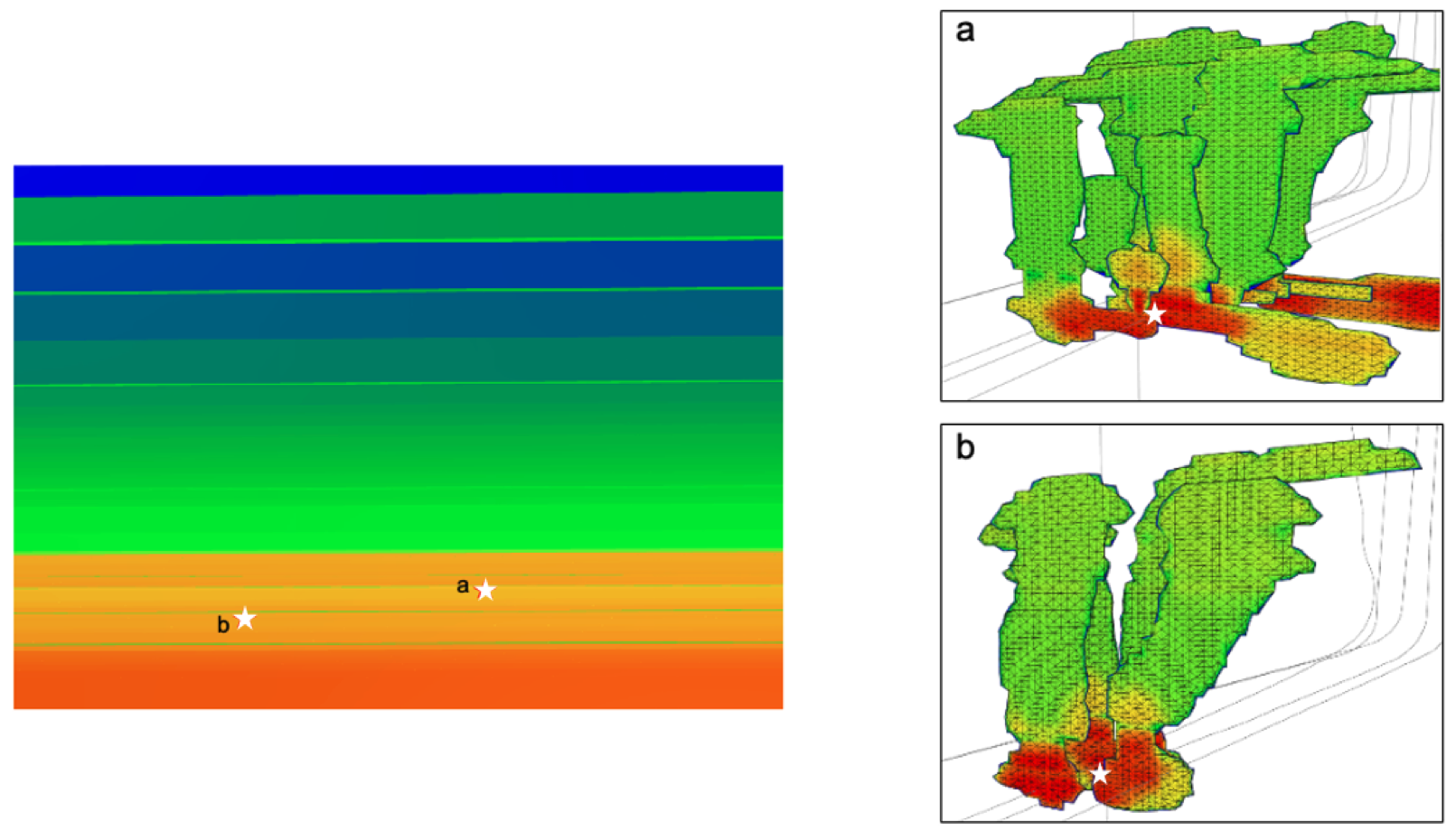
The variation of minimum principal stress with depth (when $S_3 = S_{hmin}$) results in preferential locations for fracture growth. Local minima of $S_3$ result in zones that favor fracture containment, while local maxima result in fracture barriers (Fig. 7.23). Hence, stress contrast controls vertical propagation of fractures. Fractures will preferentially grow towards regions of low stress and may stop at fractures barriers depending on the net pressure in the fracture. The fracture height $h_f$ is approximately the distance between the fracture barriers.

Figure 7.23: Example of fracture containment as a result of mechanical stratigraphy: (top) without stress contrast and (bottom) with stress contrast and determination of fracture heigth $h_f$. Inset figures from Oilfield review - Brady et. al 1992.

Horizontal stresses depend on rock properties, tectonic stress, and limits imposed by neighboring faults. Variations of horizontal stress with depth can be approximated by constructing a one-dimensional heterogeneous Mechanical Earth Model (MEM). This model consists in calculating stresses by applying a tectonic strain to a sequence of rock layers with data obtained from well logging and the laboratory. The workflow is the following (See Fig. 7.24):

1. Obtain rock mass density $\rho_{bulk}(z)$, elastic P-wave velocity $V_P(z)$, and elastic S-wave velocity $V_S(z)$ as a function of depth for a given location. You will need acoustic logging measurements which usually report travel times or slowness (units of inverse of velocity: [$\mu$s/ft]) $\Delta t_P = V_P^{-1}$ and $\Delta t_S = V_S^{-1}$.

2. Calculate the Young's modulus and Poisson's ratio (both as a function of depth) using elastic wave velocities according to the following equations:

   $$E_{dyn} = \rho_{bulk} V_S^2 \left( \frac{3V_P^2 - 4 V_S^2} {V_P^2 - V_S^2} \right)$$ (7.23)

   $$\nu_{dyn} = \frac{V_P^2 - 2 V_S^2}{2 \left( V_P^2 - V_S^2 \right)}$$ (7.24)

3. Calculate (quasi-)static Young's modulus $E_{sta}$ of the rock as a function of depth. The Young modulus calculated with elastic wave velocity $E_{dyn}$ is usually larger then the static Young's modulus $E_{sta}$ of the rock relevant to tectonic strains and strains imparted by hydraulic fracturing. The static Young's modulus $E_{sta}$ can be better approximated by laboratory measurements imparting large strains. Laboratory measurements can also measure the dynamic Young's modulus and permit establishing a relationship that links the two quantities

   $$E_{sta} = F_{ds} E_{dyn}$$ (7.25)

   where $F_{ds}<1$ is a parameter in the laboratory and usually varies from 0.3 to 0.8. The dynamic to static correction is usually done only for the Young modulus, thus, the Poisson's ratio remains the same $\nu_{sta}=\nu_{dyn}$.

4. Calculate total vertical stress $S_v$ and pore pressure$P_p$.

5. Utilize Eqs. 3.34 to calculate $S_{Hmax}$ and $S_{hmin}$ using a known tectonic strains $\varepsilon _{Hmax}$ and $\varepsilon_{hmin}$, and the static plane- strain modulus as a function of depth $E'_{sta}$. The result is what is known as a “stress log”.

Figure 7.24: Simplified workflow to calculate a stress log from wellbore logging data, field tests, and laboratory tests. The stress log permits identifying variation of horizontal stresses with depth and potential hydraulic fracture barriers.

The values of tectonic strain are usually unknown. Other measurements such as fracture tests and breakout widths along the wellbore are used to calibrate the values of tectonic strains, so that the calculated stresses match the $S_3$ values and $w_{BO}$ measured in the well.

Fig. 7.25-a shows an example of a stress log following the proposed procedure. Fig. 7.25-b-c show the results of numerical simulation of hydraulic fracture propagation started at the perforation interval shown in the stress log. Notice that the fracture avoids high stress regions, grows towards regions of low stress, and preferentially grows in regions of local stress minima.

Figure 7.25: Stress log example and fracture width from Adachi et al. [2007]. The fracture is not a simple 3D surface. Fracture width and length vary with depth. The fracture grows preferentially in at depths were minimum principal stress presents local minima.

7.4 Multistage hydraulic fracturing

The objective of multistage hydraulic fracturing is to increase the surface area of the reservoir in contact to the wellbore. Proppants help keep high conductivity in the newly created fractures. The main target of multistage hydraulic fracturing are hydrocarbon source rocks. Other hydrocarbon-bearing tight formations can be also stimulated through multistage hydraulic fracturing. An introductory animation video from Marathon is available here: https://www.youtube.com/watch?v=VY34PQUiwOQ.

7.4.1 Increased surface area with multiple fractures

Horizontal wellbores help create multiple fractures from a single wellbore whenever $S_3 = S_{hmin}$. Either for normal faulting or strike-slip regimes (and assuming $S_v$ is a principal stress - see Fig. 7.26):

• stimulation will result in a long and single fracture along a horizontal wellbore drilled in the direction of $S_{Hmax}$, and
• stimulation will result in multiple fractures perpendicular to a horizontal wellbore drilled in the direction of $S_{hmin}$.

Figure 7.26: Ideal hydraulic fracture geometry in horizontal wellbores depending on the direction of the wellbore with respect to the direction of least principal stress $S_3$.

The simplest models of hydraulic fracturing assume planar bi-wing fractures from each stage. This geometry permits defining one more parameter in addition to $(x_f, h_f, w_0)$: the distance between fracture stages $l_f$ (Fig. 7.27). One may think that reducing $l_f$ is better to increase surface area. However, placing stages too close may cause non-planar fractures to bump into each other and also require more investment. The following subsection deals with this topic. Placing a large number of fractures will require most times increasing the wellbore length. This is another design parameter, the length of the lateral $l_l$.

Figure 7.27: Ideal hydraulic fracture geometry in horizontal wellbores with least principal stress $S_{hmin}$. The distance between stages $l_f$ and the length of laterals $l_l$ (or number of stages) are two more geometrical parameters to determine.

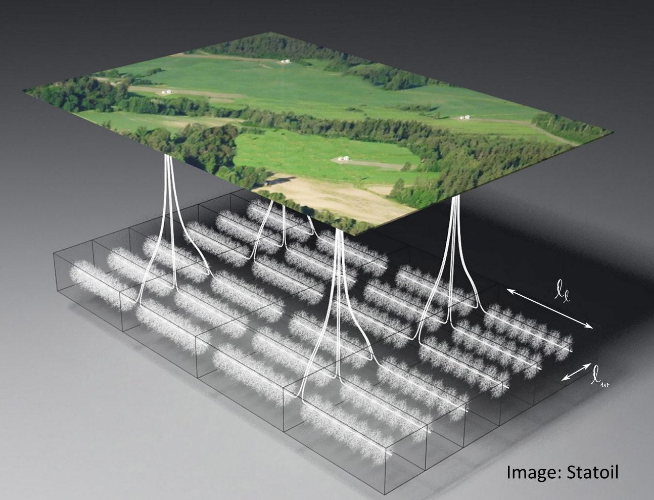
Last, usually multiple horizontal wellbores are drilled next to each other to cover the reservoir volume. Wells are usually placed parallel to each other and at the same depth spaced by inter-wellbore distance $l_w$ (Fig. 7.28). In thick formations, wells may be placed at different alternating depths. The location on surface from where the wellbores are drilled and fractured is called a drilling/fracturing pad.

Figure 7.28: Drilling/fracturing pads minimize surface utilization for multistage hydraulic fracturing. The distance between wellbores $l_w$ has to be previously calculated to maximize NPV.

Multistage hydraulic fracturing in reverse faulting may require vertical wellbores instead of horizontal wellbores. Several source rocks in Argentina, China, and Australia are subjected to mixed reverse faulting and strike-slip conditions changing with depth. The hydraulic fracturing geometry is less straight-forward in these places than in others with well defined normal faulting regime.

7.4.2 Fracture interference and fracture hit

Multistage hydraulic fracturing involves multiples fracture spaced at a characteristic distance between fractures $l_f$. This distance can be attempted by placing one fracture per stage. Hence, the distance between fractures is designed to be the distance between stages. However, if fractures are forced to grow to close to each other, they will interact due to the strains caused by placing a fracture prior to the other (Figure 7.29). The change of stress around a fracture is often referred in practice as “stress shadow”.

The minimum distance $l_f$ at which two consecutive planar fractures can be placed depends on:

• fracture propped width or equivalent net pressure,
• fracture height
• formation (rock) stiffness
• differential stress $S_2-S_3$ ( $S_{Hmax}-S_{hmin}$ in normal faulting stress regime)

The solution of change of stress due to placement of an infinitely long fracture (in direction $y$) is shown in Figure 7.29. This is Sneddon's solution for stresses around an elliptical crack in plane-strain (plane $x-z$). A net-pressure $p_{net}$ higher than the difference between the differential stress $S_2-S_3$ ($S_2$ in direction $y$ and $S_3$ in direction $x$) can make the principal stresses change directions so that $S_3$ may change to direction $y$ in the vicinity of the fracture.

Figure 7.29: Fracture interference [Make your own].

Hence, the distance $l_f$ at which a new consecutive fracture may be placed is

$$l_f \propto \frac{p_{net} h_f}{S_2-S_3}$$ (7.26)

where $p_{net}$ is proportional to the fracture width and rock stiffness ($E'$). The exact value depends on the full solution of stress around a fracture (Fig. 7.29 is a simplification). Typical net pressures are in the order of a few-hundred-psi, and the differential stress varies from location to location. Places with small stress anisotropy ( $S_2-S_3 \sim 100$ psi) are prone to significant fracture interference.

Fig. 7.30 shows an example of fracture trajectory simulation taking into account “stress shadows”. In this example the fracture width is fixed to 4 mm, which results in $p_{net} >$ 150 psi higher than $S_{Hmax}-S_{hmin} =$ 100 psi. Hence, stress rotation occurs when fractures are placed too close. In this particular example $l_f < h_f$ results in non-planar fractures that do not extend to the desired fracture direction and length as expected.

Figure 7.30: Fracture interference example for consecutive fracturing. Example for Barnett Shale, Depth = 7,000 ft, $S_{Hmax}$ = 6,400 psi, $S_{hmin}$ = 6300 psi, Pay zone 300ft ($=h_f$), fracture width = 4 mm ( $p_{net} > 150 psi$) [after Roussel and Sharma, 2011 - SPE 146104]. (a) Negligible fracture interference with $l_f =$ 400 ft. (b) Significant fracture interference with $l_f =$ 250 ft.

A practical alternative to avert the effects of stress shadows is “zipper fracturing”, which involves three or more parallel wellbores and alternate sequencing to cancel out stress shadow effects (Fig. 7.31). The idea is to reduce fracture spacing by placing fractures (e.g. number 3) only after nearby fractures have been made and propped in adjacent wells (1, 2, 1', and 2'). Sometimes, fractures in one well may run into another fractured well. This is called a “fracture hit”. Optimizing wellbore spacing, stage separation and sequencing is critically important to maximize the NPV of multistage fracturing completion work.

Figure 7.31: Zipper fracturing example [after Roussel and Sharma, 2011 - SPE 146104].

Recent completion designs give more “freedom” to fractures to develop by placing multiple perforation clusters in a single stage (Fig. 7.32). This design is called “multicluster fracturing”. The result is that fractures compete with each other to grow in the relatively close to each other. Sometimes, stress interference may halt the propagation of nearby fractures resulting in long and short fractures. In some sense, this design favors “survival of the fittest” rather than enforcing a given spacing between fractures.

Typical modern designs of multicluster fracturing in the Permian Basin have:

• length of the lateral $l_l >$ 10,000 ft,
• 40 stages,
• 4 to 15 perforation clusters in each stage,
• 6 perforations/ft in every cluster offset at 60$^{\circ }$,
• injection rate of 2 bbl/min/perf, typically averaging 100 bbl/min and a total of 60 bbl/LF (LF: linear foot of horizontal wellbore), and
• total proppant of 2,000 lb(proppant)/LF, which results in about 0.8 lb(proppant)/gallon(frac fluid).

Figure 7.32: Schematic of multicluster fracturing.

7.4.3 Fracture reactivation, microseismicity, and optical fiber monitoring

So far, we have assumed hydraulic fractures are single fractures with no branching or bifurcation. This is a conceptual and idealized shape of fluid-driven fractures.

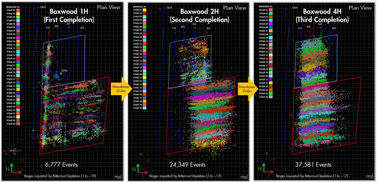
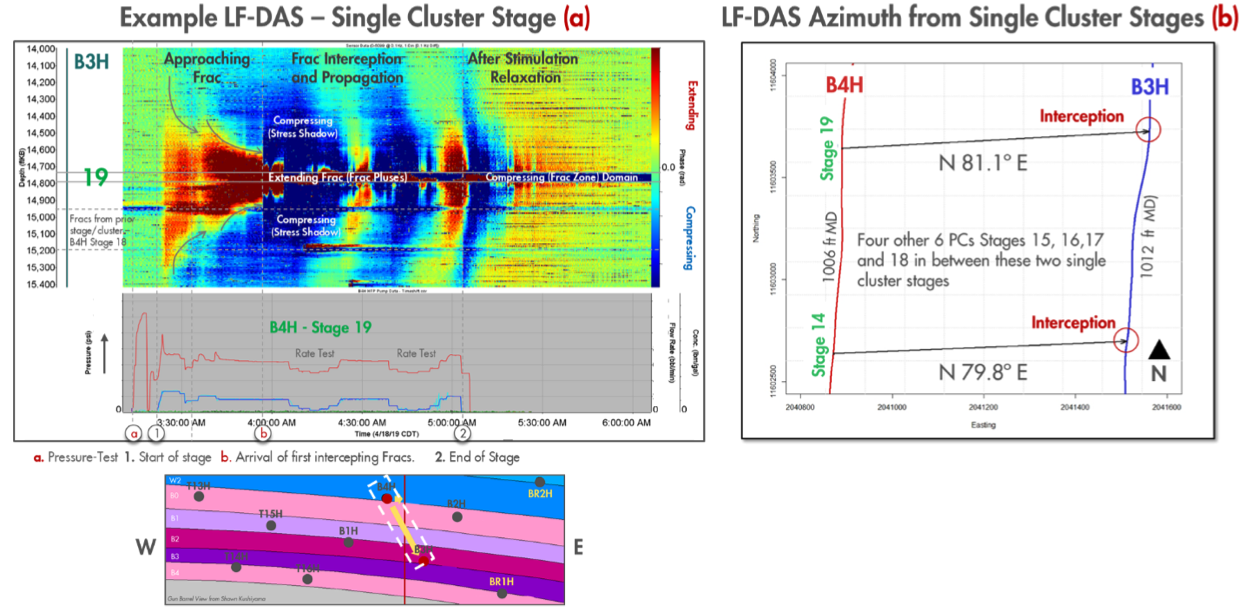
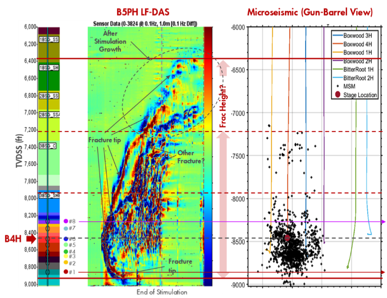
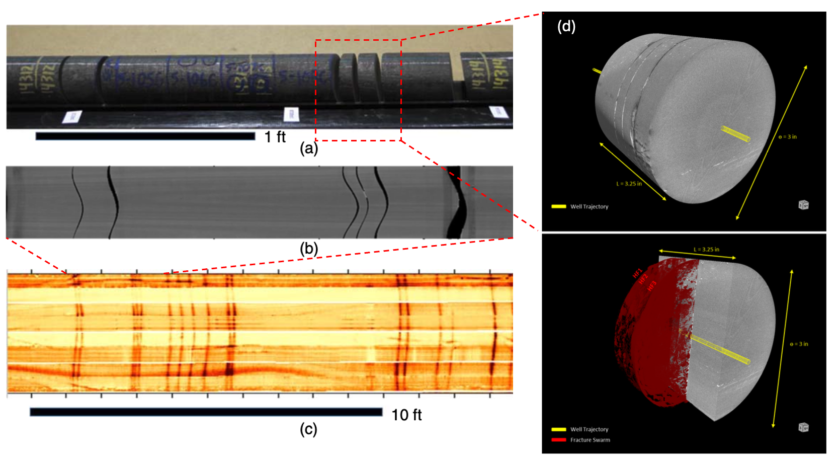
Modern monitoring tools permit observing that the rock fails in shear around hydraulic fractures. Hence, hydraulic fracturing seems to create (or re-activate) other fractures in addition to the main hydraulic fracture (Fig. 7.33).

Figure 7.33: Fracture branching idealization.

The evidence for these new fractures consists of elastic waves generated during failure (shear slippage) captured as seismic activity on geophones installed on surface and in observation wells (Fig. 7.34). The seismic activity generated from hydraulic fracturing has a magnitude usually lower than $M_L<0$ in the Richter scale (https://en.wikipedia.org/wiki/Richter_magnitude_scale), and thus is termed “microseismicity”. However, larger seismicity magnitude has been observed in some places and it is often due to fracturing fluids reaching a major fault that might have not been identified previously. Other major seismicity is often the result of continuous injection of waste water, rather than injection during hydraulic fracturing per-se.

Figure 7.34: Microseismicity idealization.

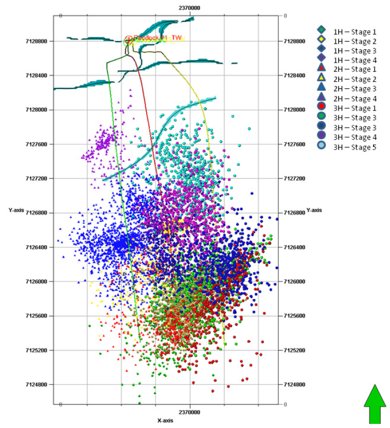
The cloud of microseismic emission is usually referred as the “Stimulated Reservoir Volume” (SRV measured in volume units). This volume is correlated to the volume that will produce hydrocarbons. The correlation is far from good, but in general, the larger the SRV, the larger the EUR. Hence, a simplified model could calculate the EUR in an unconventional oil formation as

$$EUR = RF \frac{ SRV \: \phi (1-S_w)} {B_{oi}}$$ (7.27)

Figure 7.35: Example of microseismic clouds for well completed at the Hydraulic Fracturing Testing Site 2, in the Delaware Basin (normal faulting). Microseismic clouds clearly show the stimulated reservoir volume (cross section observed here) for each stage and well. The clouds show fractures which propagate with an azimuth of about N80$^{\circ }$E, hence, $S_hmin$ local orientation is about N10$^{\circ }$W. The fractures grow preferentially towards the East, because there were already depleted wells to the East of the newly completed wells. Image credit: https://doi.org/10.15530/urtec-2021-5396 and https://netl.doe.gov/node/6840.

Figure 7.36: Example of optical fiber monitoring for hydraulic fracturing. In this example, Stage 19 in well B4H is fractured, and fiber installed along well B3H detects its arrival by fiber stretching and contraction. The plot shows strain changes from MD 14,000 to 15,400 ft (vertical axis although it is horizontal length) with time (horizontal axis). The hydraulic fracture stretches the rock and fiber at the observation well as the tip approaches (red color). The fiber contracts when the fracture tip has passed or the stimulation finishes. Image credit: https://doi.org/10.15530/urtec-2021-5396 and https://netl.doe.gov/node/6840.

Figure 7.37: Comparison of optical fiber and microseismic monitoring in a vertical cross section during stimulation of well B4H at HFTS2. The microseismic cloud (right) indicates stress perturbations up to 7,200 ft TVDSS, yet microseismic activity cannot conclusively tell whether this is a hydraulic fracture or “dry” shear reactivation only. The optical fiber shows significant strains along a vertical monitoring well B5PH up to 6,400 ft TVDSS. The monitoring suggest “buoyant” hydraulic fracture growth up to 2,000 ft above the stimulation depth, growing aseismically from 7,200 to 6,400 ft TVDSS. Image credit: https://doi.org/10.15530/urtec-2021-5396 and https://netl.doe.gov/node/6840.

Figure 7.38: Simulation example of a buoyant hydraulic fracture, where well landing and stimulation depths a and b (left figure), result in fractures propagating preferential upwards (right figures) into layers of lower minimum horizontal stress $S_{hmin}$ (in green in left figure). Te fractures grow upwards until partially stopped by the local fracture barrier (blue layers) and pumping stops. The variation of stresses with depth and across lithological units is usually known as mechanical stratigraphy. Image credit: https://doi.org/10.15530/urtec-2022-3722883. Simulation software: https://www.resfrac.com.

7.4.4 Multiple strands in hydraulic fracture propagation

Figure 7.39: Example of hydraulic fractures observed in cores retrieved from hydraulically fractured shales. Opposite to the common conception, multiple closely-spaced and semi-parallel fractures occur from a single cluster. These sets of fractures are usually referred as “fracture swarms” and the region where they preferentially propagate as “fracture corridor". The fracture corridor usually stays localized and obeys perpendicularity to the least principal stress. Subfigures a, b and c are: actual photo, unwrapped CT radial scan, and unwrapped borehole image from an example in the Eagle Ford shale (Image credit: https://doi.org/10.2118/191375-PA). Subfigure d shows a 3-fracture swarm from the Wolfcamp Shale in the Delaware Basin, where the bottom image shows digitally highlighted fractures (Image credit: https://doi.org/10.15530/urtec-2022-3709572)

.

7.5 Practical aspects of hydraulic fracturing

Figure 7.40: Schematic of field implementation.

Figure 7.41: Example of pumping and proppant schedule.

To keep in mind:

1. Fracture should remain open, hence proppant is needed.
2. Lower fluid viscosity makes fluids easier to pump.
3. Several swimming pools may be pumped in a HF treatment.
4. The power of pumps can add up to 100s of muscle cars.

7.6 Problems

1. The following data corresponds to a leak-off test in an offshore well in the Gulf of Mexico (SPE-59123-MS).
   1. Estimate $S_v$ at the shoe depth (TVDSS = 8,050 ft).
   2. Assuming the pore pressure is $P_p$ = 4,700 psi, and fracture closure occurs at time 1:18:00 (use downhole pressure reading), calculate effective vertical stress $\sigma _v$ and minimum effective stress $\sigma _3$.
   3. Calculate the effective stress anisotropy ratio $\sigma_v / \sigma_{hmin}$. What is the faulting regime?
   4. What is the density of the drilling mud?
   

2. Download the file MicrofracData.dat which corresponds to a minifrac field test. The pressure reading corresponds to surface pressure.
   1. Plot surface pressure and injection rate in a double y-axis plot as a function of time. Plot the entire interval and make a zoom from 70 to 90 min.
   2. Find the instantaneous shut-in pressure (ISIP) and make a plot of surface pressure as a function of square root of time. Find the fracture closure pressure (FCP) [surface pressure].
   3. The true depth is 7,503 ft. Assuming a hydrostatic pressure gradient inside the wellbore of 0.44 psi/ft, calculate the minimum total principal stress $S_3$ in this place.

3. The figure below shows the results of a DFIT test (data from Zoback [2007]).
   
   1. How many barrels of fracturing fluid were used in this test?
   2. Indicate fracture propagation pressure (FPP), instantaneous shut-in pressure (ISIP) and fracture closure pressure (FCP) (as well as you can without analyzing the data in detail).
   3. Describe and sketch the flow behavior around the wellbore before and after shut-in.
   4. At surface pressure of 0 psi the bottom-hole pressure is 5,500 psi. What is the minimum principal stress in this formation?

4. Interpret the following step-rate test data (i.e., find the formation parting rate and pressure). Plot pressure vs. time for all steps.
   

5. Download the file LostHills.xls. At every depth data point along the vertical well:
   1. Compute total vertical stress as a function of depth (you may assume homogeneous rock above 1750 ft), and compute overpressure parameter.
   2. Compute dynamic Poisson's ratio and dynamic Young's modulus from compressive and shear slowness (be careful with unit conversion).
   3. Compute static Young's modulus using a coefficient $E_{static} = 0.65 E_{dynamic}$.
   4. Compute static plane strain modulus $E'_{static} = E_{static} / (1-\nu^2)$ (Use dynamic Poisson's ratio ).
   5. Compute total maximum and minimum horizontal stress assuming theory of elasticity and $\varepsilon_{Hmax} = 0.0015$ and $\varepsilon_{hmin} = 0$.
   6. The pay-zone is between 2,100 ft and 2,450 ft. A hydraulic fracture is planned to be executed with a vertical well and perforations at a depth between 2,130 ft and 2,160 ft. What will be the height of this fracture? Will it reach out to the entire pay zone?

6. A single hydraulic fracture treatment will be performed in a tight sandstone. The hydraulic fracture height is expected to be $h_f$ = 170 ft. The tight sandstone has a plane-strain modulus $E'= 8.9 \times 10^6$ psi. The (two-wing) injection rate will be 50 bbl/min (constant) during 1 hour. The fracturing fluid has a viscosity 2 cP. Compute:
   1. The expected fracture half-length $x_f$, fracture width at the wellbore $w_{w,0}$, and net pressure $p_{net}$ as a function of time with the PKN model (no leak-off).
   2. The total amount of water (volume) and sand (weight) required assuming a constant volume ratio 90% water-10% sand. How many water swimming pools (100,000 L) and sand trucks (10 metric tons) are needed to complete the hydraulic fracturing job?
   Advice: convert all quantities to the SI system first.

7. Consider the design of a completion job with horizontal wellbores and multistage hydraulic fracturing in the Barnett shale at 8,200 ft with pore pressure of 4,100 psi (NF).
   1. What is the direction of horizontal wellbores that maximize drainage area using multistage fractures? (You may need to check the US stress map https://www.nap.edu/openbook/13355/xhtml/images/p45.jpg)
   2. Sketch a horizontal well with 10 fracture stages spaced every 200 ft from a top view. Fracture half-length is 500 ft.
   3. Calculate a lower bound (absolute minimum) of the pressure needed to propagate hydraulic fractures using the theory of elasticity ($\nu$=0.25) and limit equilibrium of faults ($q= 3.5$). Perforations will be done, so you may ignore the effect of near-wellbore stresses.
   4. Draw the “path” of wellbore orientation on a semi-sphere projection. The wellbore starts vertical on the surface and deviates close to the pay zone until it gets horizontal.

8. The following figures correspond to microseismicity images from hydraulic fracturing stimulation in the Barnett shale (Hydraulic Fracturing Insights from Microseismic Monitoring – SLB Oilfield Review https://www.slb.com/~/media/Files/resources/oilfield_review/ors16/May2016/02-microseismic.pdf).

   Figure 7.42: Caption from original publication “Stimulation process performed on the three horizontal wells using plug-and-perf and slickwater treatment with fault traces mapped at laterals depth interval in cyan. The zipper-style frac performed on the 1H (central well in red) and the 3H (east well in yellow) was monitored from 2H (west well in green). The four stimulation stages performed on the 2H were monitored from the 3H.”

   
   1. What is the length of the laterals? What is the spacing between laterals? What is the approximate spacing between stages? (axis units: feet) Note: 1H is 80 ft higher in elevation than 2H and 3H.
   2. What is the strike of the hydraulic fractures at the toe of the laterals? How does the strike interpreted from microseismicity compare to the strike obtained in problem 7?
   3. What is the average fracture half-length $x_f$ as interpreted from the microseismic cloud?
   4. Assuming a pay zone thickness of 200 ft, what is the Stimulated Reservoir Volume [ft$^3$]?
   5. Compute the EUR assuming a porosity of 0.1, a recovery factor of 0.1, water saturation of 0.2 and a formation volume factor of 1.2.
   6. Multiply the EUR times the price of a WTI oil barrel today (make sure you do the appropriate unit conversion). Disregarding cash flows and taxes, and assuming the costs for drilling, completion and operation are $10,000,000, is this project profitable at first glance?

7.7 Suggested Reading

• Valko and Economides, Hydraulic Fracture Mechanics, Wiley.
• Adachi, et al., (2007), “Computer Simulation of hydraulic fractures”, IJRMMS.
• Brady et al., (1992), “Cracking Rock: Progress in Fracture Treatment”, Oilfield Review. https://connect.slb.com/~/media/Files/resources/oilfield_review/ors92/1092/p04_17.pdf