Next: About this document ... Up: Introduction to Energy Geomechanics Previous: 7. Hydraulic fracturing Contents
Reservoir depletion requires changes of pore pressure.
A decrease of pore pressure
 results in increased effective stress in the depressurized region.
Effective stresses increase because the overburden
results in increased effective stress in the depressurized region.
Effective stresses increase because the overburden  remains constant above the reservoir but the pore pressure decreases.
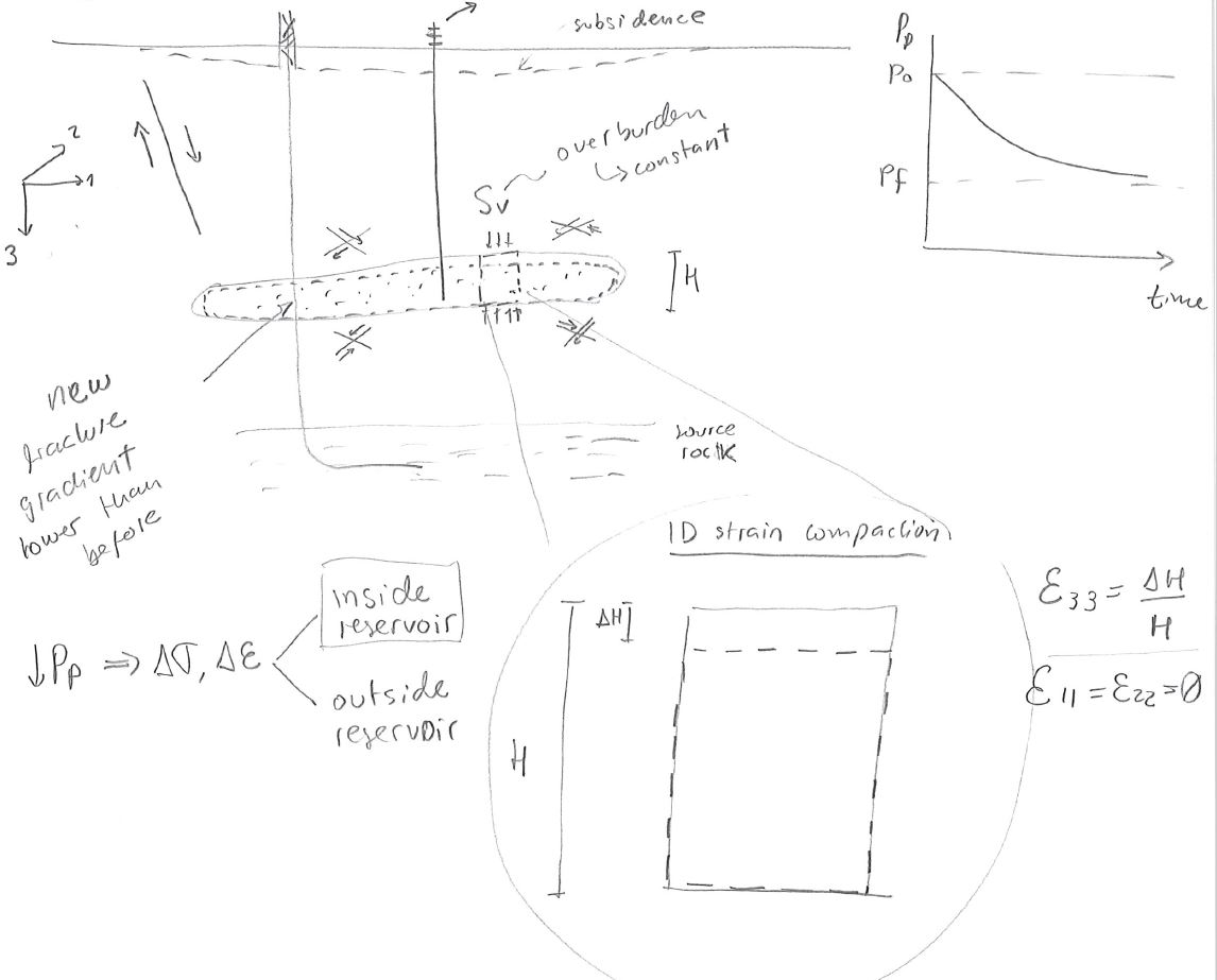
The result is compaction of the reservoir (Fig. 8.1).
Such deformation also affects neighboring formations and faults.
Changes in ground surface elevation are refered as “subsidence".
Differential displacements (for example across a fault) can result in casing damage and shearing.
Significant compaction in the reservoir layer can result in casing buckling.
The reduction of pore pressure also causes a reduction of total horizontal stress within the reservoir.
remains constant above the reservoir but the pore pressure decreases.
The result is compaction of the reservoir (Fig. 8.1).
Such deformation also affects neighboring formations and faults.
Changes in ground surface elevation are refered as “subsidence".
Differential displacements (for example across a fault) can result in casing damage and shearing.
Significant compaction in the reservoir layer can result in casing buckling.
The reduction of pore pressure also causes a reduction of total horizontal stress within the reservoir.
Reservoir depletion in horizontal, laterally extensive and thin reservoirs approximates to a one-dimensional-strain stress path, i.e. there is change in strain only in the vertical direction (Fig. 8.1). Such stress path results in increased effective stresses in both vertical and horizontal directions.
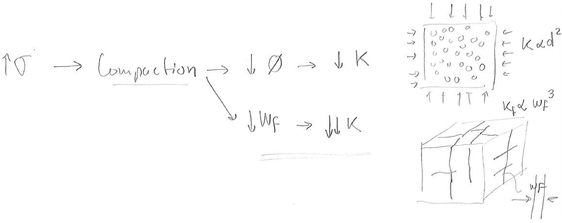
Increased effective stresses result in reduction of porosity and permeability in most cases.
The permeability of fractured rocks tends to be more sensitive to stress than typical rock matrices.
The reason is that permeability is proportional to the
 in rock matrix, while permeability is proportional to the
  in fractures (Fig. 8.2).
The variability of rock permeability with stress is called “fracture compressibility".
The decline curves of unconventional formations are highly influenced by fracture compressibility.
in fractures (Fig. 8.2).
The variability of rock permeability with stress is called “fracture compressibility".
The decline curves of unconventional formations are highly influenced by fracture compressibility.
Let us use the theory of poroelasticity (Section 3.7.1) to solve for the changes of total and effective stresses with depletion.
According to this theory, effective stress must be corrected for the Biot coefficient  so that,
 |
(8.1) |
We use this equation of effective stress together with linear isotropic elasticity in order to relate stresses to strain (
 , and the assumption of one-dimensional strain
![$\uuline{\varepsilon} = [0,0,\varepsilon_{33},0,0,0]^T$](img414.svg) (3-vertical direction):
(3-vertical direction):
The equation corresponding to the 3rd row results in:
 |
(8.3) |
The denominator is the constrained modulus
 .
Hence, the vertical strain in the reservoir layer is:
.
Hence, the vertical strain in the reservoir layer is:
 |
(8.4) |
Remember that  is the overburden stress and does not change with time or with reservoir pore pressure.
Notice that depletion (
is the overburden stress and does not change with time or with reservoir pore pressure.
Notice that depletion (
 ) results in compaction (
 ).
This deformation is linked to the reservoir compressibility.
Hence, according to linear poroelasticity the uniaxial bulk compressibility is
).
This deformation is linked to the reservoir compressibility.
Hence, according to linear poroelasticity the uniaxial bulk compressibility is
 (See Section 3.3.5).
Combining Equations from rows 1 and 3 (or 2 and 3), results in
Depletion (
) results in decreases of horizontal stress (
 ).
The same change of stress occurs in direction 2.
The coefficient of proportionality in the previous equation is usually referred as
).
The same change of stress occurs in direction 2.
The coefficient of proportionality in the previous equation is usually referred as
 and varies typically from 0.5 to 0.9.
The prediction of
and varies typically from 0.5 to 0.9.
The prediction of  can be validated through hydraulic fracture tests that measure minimum horizontal total stress
  in places with normal faulting and strike slip regime.
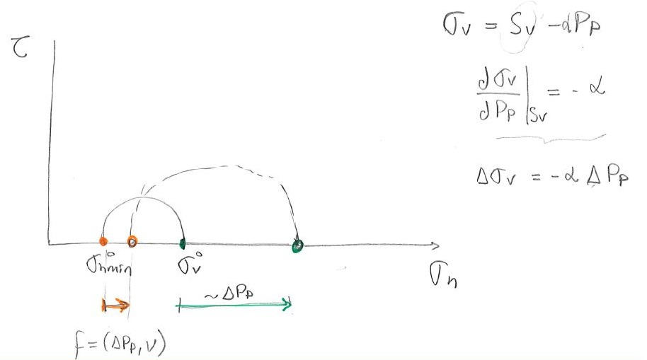
A total stress path plot describes the value of total stresses as a function of pore pressure (Fig. 8.3).
![\includegraphics[scale=1.05]{.././Figures/split/10-TotalStressPath.pdf}](img1239.svg) |
Depletion results in increased effective stresses.
The change of vertical effective stress
 (with constant) is
 |
(8.6) |
From Equation 8.5, the change of horizontal effective stress with pressure is
 |
(8.7) |
Both, horizontal and vertical effective stresses increase with depth. This results in a shift of the Mohr circle to the right and up, i.e. increased mean effective stress and increased deviatoric stress (Fig. 8.4). Large compressive and shear stresses can result in rock failure under compression and shear. Grain crushing can significantly decrease the rock permeability.
 |
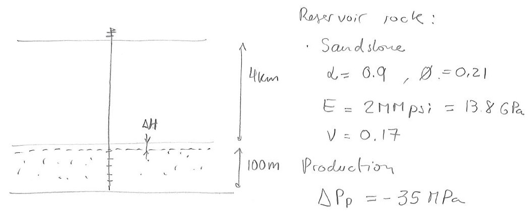
PROBLEM 8.1: Calculate the following due to depletion of 35 MPa.
 at the top of the reservoir.
 .
.
 .
.
 and horizontal stresses
 .
.
 with the following law (
 MPa
MPa ):
):
![$\displaystyle k = k_o \: \exp \left[ -c_f (\sigma_h - \sigma_h^o) \right]$](img1249.svg) |
SOLUTION
 GPa GPa |
 , where
 |
 m
m  m.
m.
 |
 |
 MPa MPa  MPa MPa |
 MPa MPa  MPa MPa |
 MPa MPa |
is
![$\displaystyle \frac{k}{k_o} = \exp \left[ -c_f (\sigma_h - \sigma_h^o) \right]
...
... -0.25 \text{ MPa}^{-1} (+6.45 \text{ MPa}) \right] \sim 0.2 \: \: \blacksquare$](img1262.svg) |
![\begin{displaymath}%compliance matrix
\left[
\begin{array}{c}
S_{11} - \alpha P...
... \cfrac{}{} \\
0 \cfrac{}{}\\
0 \cfrac{}{}
\end{array}\right]\end{displaymath}](img1229.svg)