3.1 Stress tensor

Consider a 3D space with a given right-handed orthogonal coordinate system $\uline{e}_1$, $\uline{e}_2$, $\uline{e}_3$ in directions 1, 2 and 3 (Figure 3.2). In a right-handed coordinate system, the first element of the base $\uline{e}_1$ is your index finger, the second element of the base $\uline{e}_2$ is your middle finger, and the third element of the base $\uline{e}_3$ is your thumb (all in your right hand).

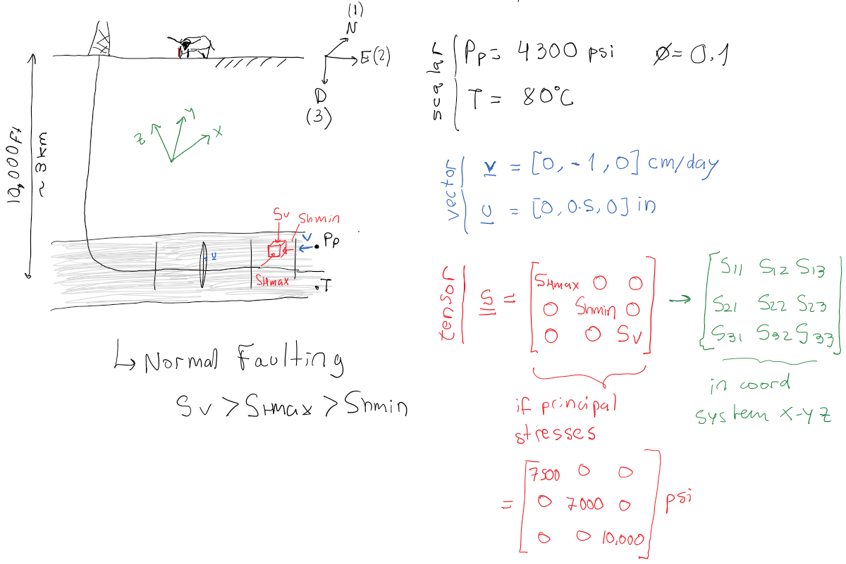
The number that represents the value of a scalar (such as temperature $T$ or pore pressure $P_p$) at a given point $(x_1,x_2,x_3)$ is independent of the coordinate system orientation and origin (Figure 3.1). However, the numbers that represent the value of a vector (such as velocity $\uline{v}$ or force $\uline{F}$) or a tensor depend on the coordinate system. A tensor, like stress, also depends on the coordinate system used to express its numerical values. Read the values $S_{ij}$ as the stress on face perpendicular to base vector $\uline {e}_i$ in the direction of base vector $\uline {e}_j$. $S_{ij}$ is positive if after a displacement $dx_i$, $S_{ij}$ points in opposite direction to $\uline {e}_j$ (Figure 3.2).

Figure 3.1: Examples of scalar, vector and tensor quantities in a shale reservoir.

All stresses $S_{ij}$ can be written as a matrix (Figure 3.2). The diagonal terms correspond to normal stresses. The off-diagonal terms correspond to shear stresses. Off-diagonal stresses are symmetric $S_{ij}=S_{ji}$ ($i \neq j$) because of angular momentum equilibrium (the element does not spin around any axis). Hence, the stress tensor is symmetric with respect to the diagonal (top-left to bottom-right).

Figure 3.2: Graphical and mathematical representation of the stress tensor. Read $S_{ij}$ as the stress on face perpendicular to $\uline {e}_i$ in the direction $\uline {e}_j$. $S_{ij}$ is positive if after a positive displacement $dx_i$, $S_{ij}$ points in direction opposite to the directions of the base element $\uline {e}_j$. All stresses in this figure have been drawn to be positive.

Since the stress tensor is symmetric and is composed by all real numbers, there exist 3 real-valued eigenvalues that we call principal stresses and denote $S_1 \geq S_2 \geq S_3$. Each principal stress (eigenvalue) is associated with a principal direction (eigenvector). Principal directions are always perpendicular to each other in a cartesian coordinate system. When we write the stress tensor in the coordinate system aligned with directions of the principal stresses, the stress tensor results in diagonal elements populated by the principal stresses and zeros in the off-diagonal places. Usually, the principal stresses are ordered from top to bottom starting with $S_1$ at the top (Figure 3.3).

Figure 3.3: Principal stresses and directions. Every tensor with non-zero off-diagonal terms can be simplified to a principal stress tensor with zero off-diagonal terms at the orientation that coincides with the directions of principal stresses.

EXAMPLE 3.1: For the following stress tensor obtained for the Neuquen Basin: a) calculate the eigenvalues (principal stresses), b) calculate eigenvectors (principal directions), c) answer what the stress regime is, and d) calculate the angle between the North and the direction of $S_{Hmax}$ in clockwise direction.

$$\underset{=}{\sigma} = \left[ \begin{array}{ccc} \sigma_{NN} ... ...ccc} 8580 & 100 & 0 \\ 100 & 9900 & 0 \\ 0 & 0 & 9000 \end{array} \right]$$   psi

Note: The stress tensor is written in the North-East-Down coordinate system.

SOLUTION
First, find an appropiate math solver that can calculate eigenvalues and eigenvectors (Python, Matlab, Wolfram Alpha, etc.) We will use Wolfram Alpha online in this solution. Go to https://www.wolframalpha.com/ and enter:

eigenvalues $\left\{ \left\{ 8580,100,0 \right\}, \left\{ 100,9900,0 \right\}, \left\{0,0,9000 \right\} \right\}$

The answer to this querry is (click in “approximate forms”):

$$\left\{ \begin{array}{ccc} \lambda_1 & = & 9907.53 \\ \l... ...2 & = & 9000 \\ \lambda_3 & = & 8572.47 \end{array} \right.$$

and

$$\left\{ \begin{array}{ccc} \nu_1 & = & (0.0753277,1,0) \\ ... ...& (0,0,1) \\ \nu_1 & = & (-13.2753,1,0) \end{array} \right.$$

a,b) The principal stresses are

$$\left\{ \begin{array}{ccc} S_{Hmax} & = & 9907.53 \text{ p... ...} \\ S_{hmin} & = & 8572.47 \text{ psi} \end{array} \right.$$

Figuring out what are horizontal and vertical stresses depends on the eigenvectors. First, let's start with the easiest one. Eigenvector $\nu_2 = (0,0,1)$ points straight in the downward direction, i.e., no horizontal component either in N or E directions (first two coordinates are zeros). Hence, $\lambda_2 = 9000$ is in the vertical direction and is $S_v$. The other two ($\lambda_1$ and $\lambda_3$) are the horizontal stresses, where $\lambda_1 > \lambda_3$ and therefore $\lambda_1 = S_{Hmax}$.

c) $S_v$ is the intermediate stress in this case, hence, this location is under strike-slip stress regime according to the Andersonian classification.

d) Eigenvector $\nu_1 = (0.0753277,1,0)$ gives the direction of $\lambda_1 = S_{Hmax}$. Let's read the vector $\nu_1$ according to the NED coordinate system: it goes North +0.0753277 units, it goes East +1.0 units, it goes Down 0.0 units. Drawing this in a 3D coordinate system results in a vector in the NE horizontal plane pointing mostly towards the East. The angle between the East axis and the vector is $\arctan (0.0753277/1) = 0.075$    rad$= 4.3 ^{\circ}$, i.e., $4.3 ^{\circ}$ from the East axis towards the North axis. Hence, the angle between the North and the vector $\nu_1$ is $90^{\circ} - 4.3 ^{\circ} = 85.7^{\circ}$. $\: \: \blacksquare$

3.1.1 Cauchy's equations of stress equilibrium

Equilibrium of stresses requires summation of forces in all directions to be zero when the object is not moving (no acceleration $\uline{a}$, thus $m \uline{a} = 0$). Consider the schematic in Figure 3.4. Summation of forces in direction 1, where the term $\rho V b_1$ is the body force component, proportional to the solid mass density $\rho$ and volume $V$, and the acceleration component $b_1$, requires

$$\begin{array}{rcl} \sum F_1 & = & 0 \\ \sum F_1 & = & + S_{1... ...] dx_1 dx_2 \\ & & - \rho (dx_1 dx_2 dx_3) b_1 = 0 \end{array}$$

which eventually reduces to the following equation when canceling terms and dividing by the element volume $(dx_1 dx_2 dx_3)$

$$\frac{\partial S_{11}}{\partial x_1} + \frac{\partial S_{21}}{\partial x_2} + \frac{\partial S_{31}}{\partial x_3} - \rho b_1 = 0$$ (3.1)

Figure 3.4: Equilibrium of forces in direction 1. $S_{21}$, $S_{31}+\frac {\partial S_{31}}{\partial x_3} dx_3$ and $S_{11}+\frac {\partial S_{11}}{\partial x_1} dx_1$ are applied on the non-visible faces of the solid element.

A generalization of equilibrium in all directions with all stresses (Figure 3.2) yields the Cauchy's equilibrium equations:

$$\displaystyle \left\lbrace \begin{array}{rcl} \cfrac{\partial... ...S_{33}}{\partial x_3} - \rho b_3 & = & 0 \\ \end{array}\right.$$ (3.2)

3.1.2 Application of Cauchy's equations for total vertical stress calculation

Consider a half-space where the surface coincides with the origin of the coordinate system and gravity $g$ points in direction 3, hence $b_3 = g$ in Eq. 3.2. We assume infinite extension in directions 1 and 2, therefore there are no variations in directions 1 and 2, such that $\partial()/\partial x_1 = \partial()/\partial x_2 = 0$. Notice there are 6 unknowns and 3 equations in Eq. 3.2 (remember $S_{ij}=S_{ji}$ ). The only equation we can solve is the third one. Integration of the third equation yields the (vertical) stress $S_{33}$,

$$S_{33}(x_3) = \int_0^{x_3} \rho(x_3) g \: dx_3$$ (3.3)

equivalent to Eq. 2.11.

Figure 3.5: Stress gradient in a solid half-space and derivation of total vertical stress $S_{33}$ as a function of depth.

You may wonder “what about $S_{11}$ and $S_{22}$? The horizontal stresses cannot be determined with the current equations. The solution to this problem will be developed in section 3.3.4.

3.1.3 Continuum mechanics solution of an arbitrary problem

Figure 3.6 shows an example of an arbitrary shaped continuous solid subjected to external stresses $\uline{t}$, external forces $\uline{F}$, body forces $\uline{b}$, and displacement constraints (bottom fixture). As highlighted before, notice that there are 6 unknowns (9 unknowns if displacements are included) and 3 equations in Cauchy's equations of equilibrium (Eq. 3.2). The solution of a general problem with arbitrary boundary conditions requires more equations to have a determined problem (as many equations as unknowns). The solution of such problem requires knowledge of the material properties. We need equations that relate displacement to stresses. These equations divide in two types:

• kinematic equations, that relate displacements to strains, and
• constitutive equations, that relate strains to stresses.

The following section describes the simplest form of kinematic and constitutive equations.

Figure 3.6: A general equilibrium problem. The solution of a general continuum mechanics problem requires knowledge of material properties and solid deformation.