5.3 Frictional strength of faults and fault types

5.3.1 Fault strength

At the large scale, the Earth's crust is constituted by “already broken" rock layers. These discontinuities are comprised mostly of faults. The cementation or cohesive strength of faults is negligible because the rock is already broken at those interfaces. Hence, a large block of rock does not have any cohesive strength or “unconfined compression strength”. As a result, its shear strength depends only on frictional strength according to the Coulomb frictional criterion (Fig. 5.11). You may think of “El Capitán” rock cliff (https://www.reviewjournal.com/wp-content/uploads/2018/06/10646363_web1_yosemite-fatal-fall_6053325.jpg) as an example of a rock mass, strong and continuous, but that is an exception, not the rule. Furthermore, the size of “El Capitán” ($\sim$ 900 m $\sim$ 3000 ft) is smaller than the size of sedimentary basins ($\sim$ 100 km and bigger).

Because of the lack of cohesive strength of the Earth's crust at the large scale, its shear strength just depends on frictional strength through the friction coefficient $\mu$ (or equivalent friction parameter $q$). The coefficient $\mu_i$ is the internal frictional angle of rock before rupture, while $\mu$ is the friction coefficient after initial rupture. Hence, the shear strength of large blocks in the Earth's crust is simply

$$\tau = \mu \: \sigma_n$$ (5.1)

which can be rewritten in terms of principal stresses as

$$\sigma_1 = q \: \sigma_3$$ (5.2)

where

$$q = \left( \sqrt{\mu^2 +1} + \mu \right) ^2 = \frac{1+\sin \: \varphi}{1-\sin \: \varphi}$$ (5.3)

For typical friction coefficients the coefficient $q$ varies from 3 to 7. This means that the maximum ratio between maximum principal effective stress and minimum principal effective stress is $\sigma_1/\sigma_3 \sim$ 3 to 7 (See Table 5.1). This ratio is usually called “(effective) stress anisotropy”.

Figure 5.11: Limits on effective principal stresses.

Table 5.1: Relationship between friction coefficients, maximum stress anisotropy, and expected failure angle.

$\mu$	$q$	$\phi$	$\pi/4 + \phi/2$
0.6	3.1	$\sim 30 ^{\circ}$	$\sim 60 ^{\circ}$
1.0	5.8	$45 ^{\circ}$	$67.5 ^{\circ}$
1.2	7.6	$50 ^{\circ}$	$70 ^{\circ}$

The maximum allowable stress anisotropy in a geological formation depends on its shear strength. Faults form or reactivate when this stress anisotropy, and therefore shear strength, is surpassed.

• $\sigma_1 / \sigma_3 > q$ implies fault slip.
• $\sigma_1 / \sigma_3 < q$ implies no fault slip.

These relationships can also be worked out in terms of total stresses but it is easier and more meaningful to keep them in terms of effective stresses (just do not forget about pore pressure).

5.3.2 Normal faults

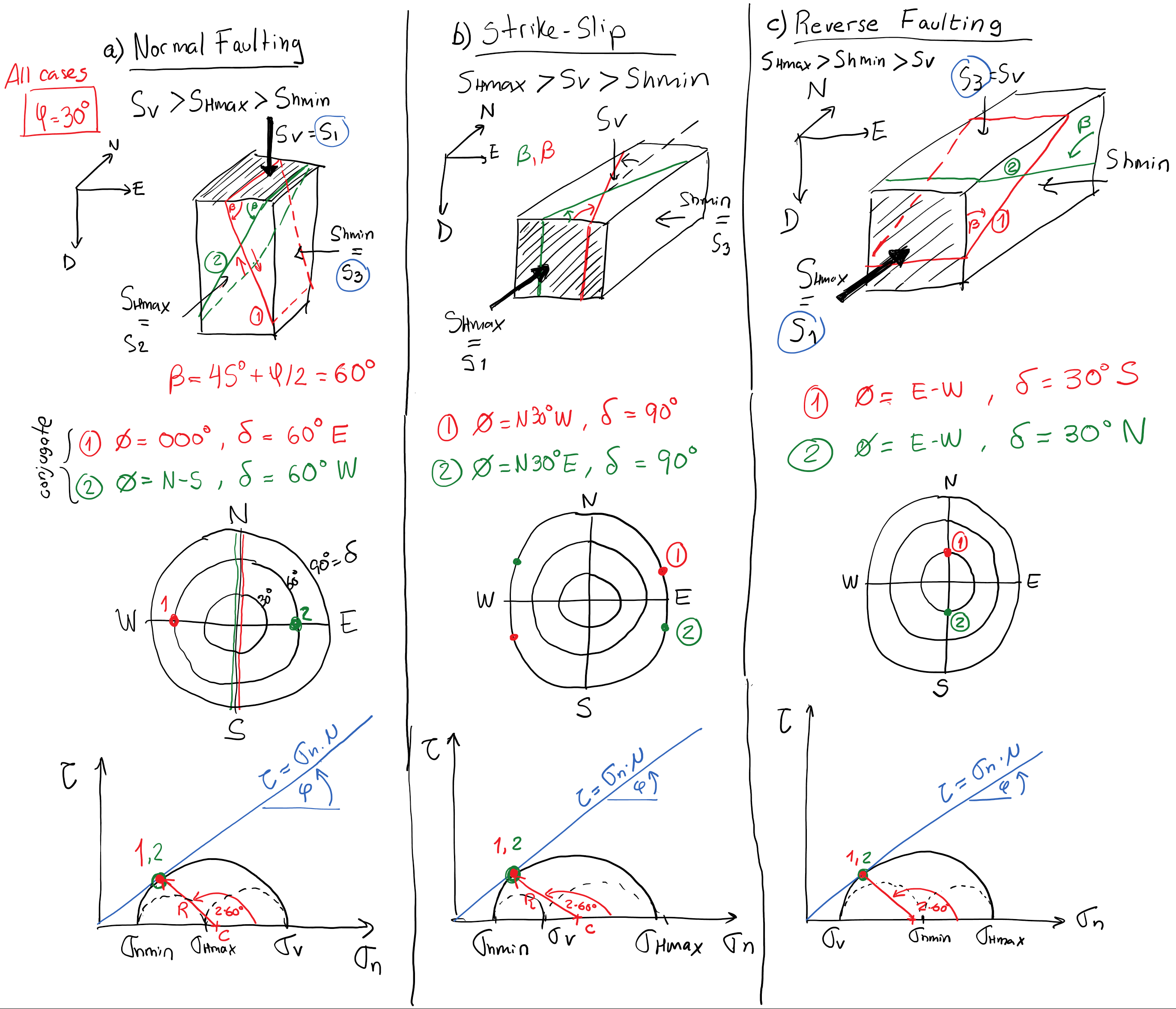
A normal fault is caused by in-situ stress conditions in which

$$\left\lbrace \begin{array}{l} S_1 = S_v \\ S_2 = S_{Hmax} \\ S_3 = S_{hmin} \\ \end{array}\right.$$ (5.4)

where $S_1 > S_2 > S_3$. These stress conditions are typical of tectonically passive and laterally extensional environments. For example, the Permian Basin in Texas is mostly under normal faulting stress regime. The fault plane is a shear rupture plane. Its orientation is ( $\pi/4 + \varphi/2$) in vertical direction from the horizontal plane (the plane perpendicular to $S_v$) to the plane of $S_{hmin}$. The blocks move along the direction of $S_v$ and do work against $S_{hmin}$. At any point in the fault, the block above the fault is called the “hanging-wall” and the block below is the “footwall” (Fig. 5.12).

Figure 5.12: Single normal fault

Normal faults usually occur in pairs. Notice that the shear failure angle includes two possible solutions (for $S_1 \neq S_2 \neq S_3$). These are called conjugate solutions. The block that moves down in between two normal conjugate faults is termed “graben”, while the ones that move up relative to the footwall are called “horst” (Fig. 5.13). These geological structures occur frequently in hydrocarbon systems with structural fault traps.

Figure 5.13: Conjugate normal faults forming graben and horst structures.

5.3.3 Thrust and reverse faults

A thrust fault is caused by in-situ stress conditions in which

$$\left\lbrace \begin{array}{l} S_1 = S_{Hmax} \\ S_2 = S_{hmin} \\ S_3 = S_v \\ \end{array}\right.$$ (5.5)

These stress conditions are typical of locations with high compressive tectonic strains. For example, sedimentary basins close to the Andes and Himalayas foothills are under reverse faulting regime. The fault plane is a shear rupture plane. Its orientation is $(\pi/4 + \varphi/2)$ in vertical direction from a vertical plane perpendicular to $S_{Hmax}$ to the plane of $S_{v}$ (Fig. 5.14). The blocks move along the direction of $S_{Hmax}$ and do work against gravity $S_v$ (surface uplift). As with normal faulting, the block above the fault is called the “hanging-wall” and the block below the “footwall”.

Figure 5.14: Thrust fault example.

A fault that may have been caused by paleo-stresses corresponding to a normal stress regime, but now moves according to in-situ stress conditions of a thrust fault stress environment is termed a reverse fault (Fig. 5.15).

Figure 5.15: Reverse fault example.

5.3.4 Strike-slip faults

A strike-slip fault is caused by in-situ stress conditions in which

$$\left\lbrace \begin{array}{l} S_1 = S_{Hmax} \\ S_2 = S_v \\ S_3 = S_{hmin} \\ \end{array}\right.$$ (5.6)

These stress conditions are typical of high compressive tectonic strains mostly in one direction. Some sedimentary basins around the Rocky Mountains and near California are under strike slip regime. The fault plane is a shear rupture plane and it is vertical. Its orientation is $(\pi/4 + \varphi/2)$ in horizontal direction from a vertical plane perpendicular to $S_{Hmax}$ towards a plane perpendicular to $S_{hmin}$. The schematic in Fig. 5.16 shows an oblique fault, not a pure strike-slip fault. The fault is called strike-slip, because it slips in horizontal direction, in the direction of the fault strike. Notice that oblique faults move with a combination of vertical and horizontal displacements.

Figure 5.16: Strike-slip fault example.

5.3.5 Stress and faulting regimes

The type of fault that occurs for each stress combination gives rise to the name of the stress faulting regime (Table 5.2). Notice that stresses may change in magnitude and direction with time at a given location (see stress map in Fig. 5.17 - other maps available at http://www.world-stress-map.org/). Furthermore, the same location may evolve through different stress regimes over geological periods of time. The stress regime can also change with depth at the same location. Changes of stress regime with depth are critical for defining the geometry of fluid-driven fractures.

Table 5.2: The Andersonian faulting classification system.

Faulting regime	Maximum principal	Intermediate principal	Minimum principal
	stress $S_1$	stress $S_2$	stress $S_3$
Normal (NF)	$S_v$	$S_{Hmax}$	$S_{hmin}$
Strike-slip (SS)	$S_{Hmax}$	$S_v$	$S_{hmin}$
Reverse (RF)	$S_{Hmax}$	$S_{hmin}$	$S_{v}$

Figure 5.17: World stress map http://www.world-stress-map.org/. The figure above shows directions of maximum horizontal stresses based on various types of field measurements. The orientation of maximum horizontal stress varies with location and is strongly influenced by plate movement and imparted tectonic strains.

5.3.6 Ideal orientation of faults

The ideal orientation of a hydraulic fracture is a plane perpendicular to the minimum principal stress $S_3$ direction. Similarly, we can also tell what would be the orientation of ideal conjugate pairs of shear fractures (faults) for a given state of stress. The dip and strike will depend on $S_1$, $S_3$, and the friction angle $\varphi$ (Fig. 5.19). Such ideal conjugate pair of shear fractures would be located:

• in planes that are in between the planes perpendicular to $S_1$ and $S_3$,
• in planes that are co-linear with $S_2$,
• in planes that are at $\pi/4 + \varphi/2$ from the plane perpendicular to $S_1$ towards the plane perpendicular to $S_3$.

The general solution is shown in Figure 5.18.

Figure 5.18: Ideal orientation of a pair of conjugate shear fractures (faults) as a function of the orientation of principal stresses and the friction angle.

Notice that all these angles vary according to the stress regime. Faults formed in NF stress regime tend to be steep. Faults formed in RF stress regime are not too steep. Faults formed in SS stress regime are vertical.

Figure 5.19: Summary of ideal pairs of shear fractures in (left) normal fault stress regime, (center) strike-slip stress regime, and (right) thrust (reverse) faulting stress regime. From top to bottom the figure shows: block diagrams with stresses, block diagram with shear fractures, stereonets, and 3D Mohr circles.

PROBLEM 5.1: Find the ideal orientation of a hydraulic fracture and faults (shear fractures) at a location subjected to the following state of stress and conditions:

• Stress regime: Normal faulting
• $S_v$ is a principal stress
• Azimuth of $S_{hmin}$ is N60$^{\circ }$W
• Friction angle $\varphi$ = 30$^{\circ }$.

SOLUTION
First, recognize the planes of $S_1$ and $S_3$ and their orientations with respect to the geographical coordinate system. The plane of $S_1$ in this case is a horizontal plane ($S_v$ plane, a principal stress) and the plane of $S_3$ is a vertical plane perpendicular to $S_{hmin}$.

A hydraulic fracture would be perpendicular to $S_3$, in this case $S_{hmin}$. Hence, the strike is $\phi_{HF} = 030^{\circ}$ and the dip is $\delta_{HF} = 90^{\circ}$ because $S_3$ is horizontal.

The dip of faults depends on the friction angle. In this case, the failure angle is:

$$\beta = 45^{\circ} + \varphi / 2 = 45^{\circ} + 30^{\circ} / 2 = 60^{\circ}$$

The fault planes are at $\beta$ going from the plane of $S_1$ to the plane of $S_3$. Thus, the strike of the two possible faults is $\phi_{F1} = \phi_{F2} = 030^{\circ}$ and the dips are $\delta_{F1} = 60^{\circ}$SE and $\delta_{F1} = 60^{\circ}$NW. $\: \: \blacksquare$

PROBLEM 5.2: Find the ideal orientation of a hydraulic fracture and faults (shear fractures) at a location subjected to the following state of stress and conditions:

• Stress regime: Strike-slip faulting
• $S_v$ is a principal stress
• Azimuth of $S_{Hmax}$ is 010$^{\circ }$
• Friction angle $\varphi$ = 40$^{\circ }$.

SOLUTION
First, recognize the planes of $S_1$ and $S_3$ and their orientations with respect to the geographical coordinate system. The plane of $S_1$ in this case is a vertical plane ($S_{Hmax}$ plane) and the plane of $S_3$ is another vertical plane perpendicular to $S_{hmin}$.

A hydraulic fracture would be perpendicular to $S_3$, in this case $S_{hmin}$. Hence, the strike is $\phi_{HF} = 010^{\circ}$ and the dip is $\delta_{HF} = 90^{\circ}$ because $S_3$ is horizontal.

The dip of faults depends on the friction angle. In this case, the failure angle is:

$$\beta = 45^{\circ} + \varphi / 2 = 45^{\circ} + 40^{\circ} / 2 = 65^{\circ}$$

The fault planes are at $\beta$ going from the plane of $S_1$ to the plane of $S_3$. Thus, the strikes of the two possible faults are $\phi_{F1} = 345^{\circ}$ and $\phi_{F2} = 035^{\circ}$, the dip is $\delta_{F1} = \delta_{F2} = 90^{\circ}$. $\: \: \blacksquare$