5.2 Mapping of faults and fractures

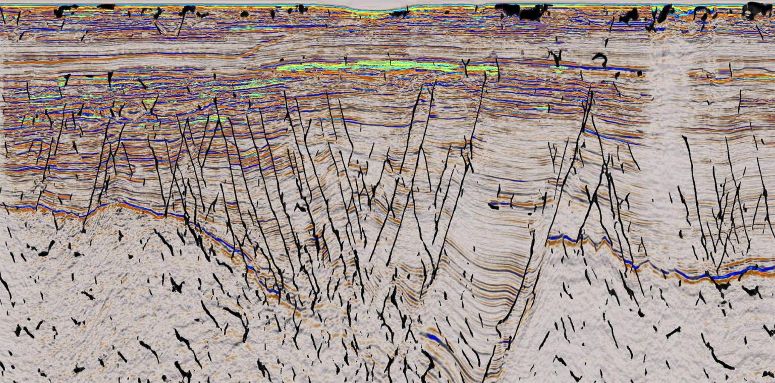
Faults in subsurface formations are usually mapped through seismic reconstruction (see example in Fig. 5.3) and wellbore imaging.

Figure 5.3: Fracture mapping in seismic images (Credit: ConocoPhillips).

Fig. 5.4-a shows the typical signature of fractures in a wellbore. An anomaly of electrical resistivity or ultrasonic P-wave velocity facilitates recognizing the fracture (dark pixels in the image). The reconstruction of this image (Fig. 5.4-b) helps measure fracture orientation (strike and dip - Fig. 5.4-c).

Figure 5.4: Fracture mapping in wellbores. [make your own]

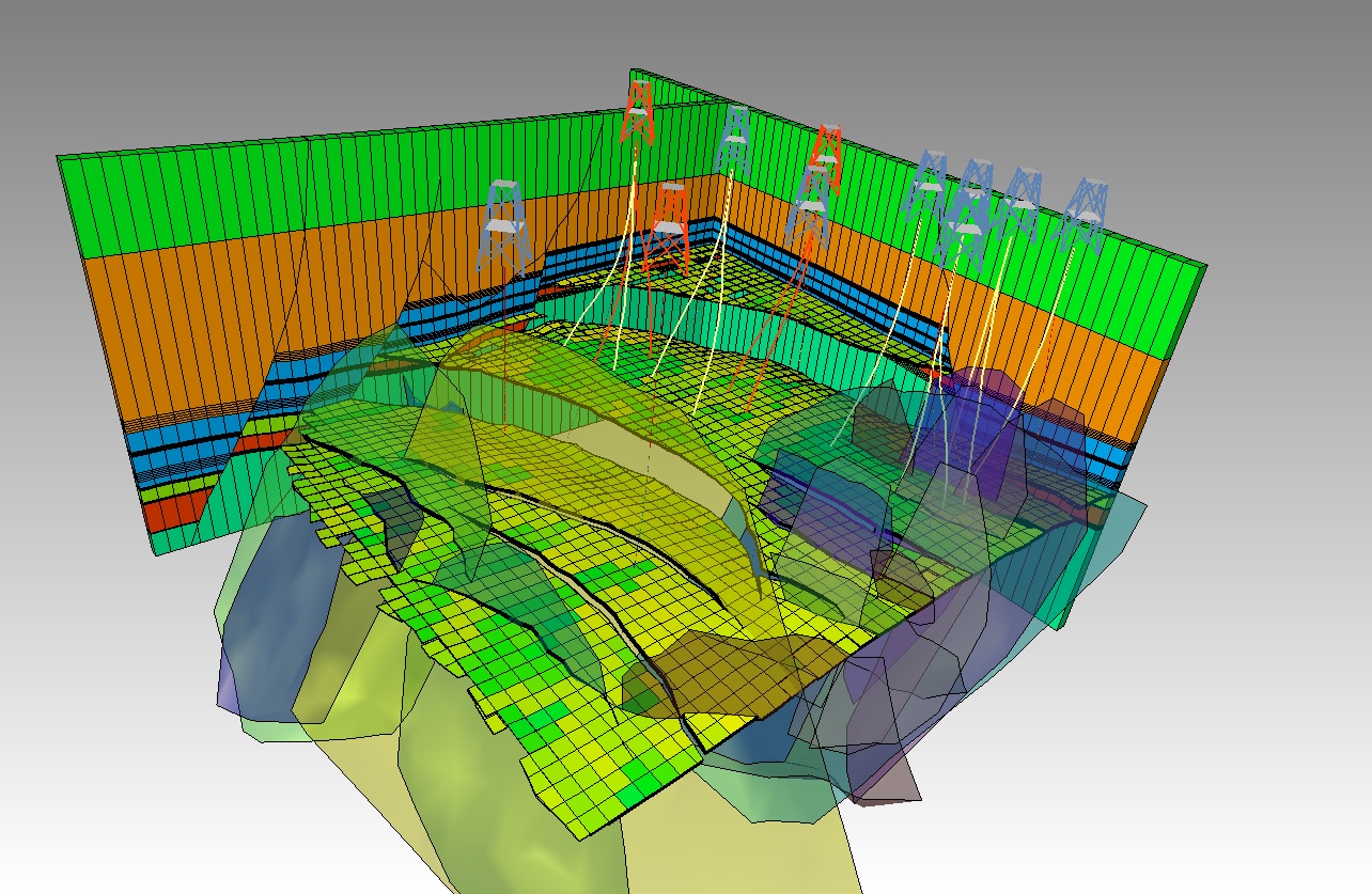
Comprehensive fracture mapping helps create 3D reservoir models that account for fault and fracture geomechanics (5.5). The magnitude of shear and normal stresses on faults and fractures depends on their orientation respect to the in-situ stress tensor.

Figure 5.5: Reservoir model example including faults (Courtesy Baker Hughes).

5.2.1 Orientation of planes with respect to the geographical coordinate system

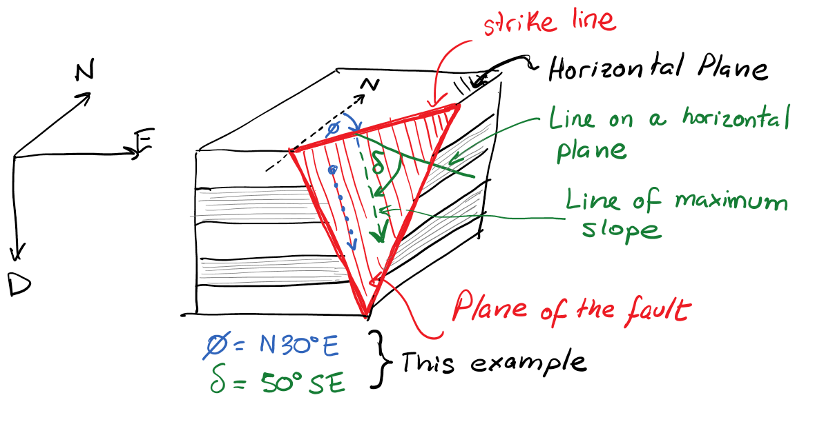
Imagine any plane (such as the plane shown in Fig. 5.6) cutting horizontal sedimentary strata. The strike is the line which results from the intersection of such plane and a horizontal plane. The magnitude of the strike is the angle between the strike line and the north. The angle of dip is the angle between a horizontal plane and the plane under consideration. A layer is said to dip in a given direction when it gets deeper at the fastest rate into such direction. One can think of the $dip$ as the direction of a droplet of water moving down on such plane.

Figure 5.6: Definition of strike and dip. [make vectorial plot]

There are two conventions for reporting the magnitude of strike.

• Quadrant convention: it reports strike with angles ranging from 0 to 45$^{\circ }$. The quadrant convention is useful in the field. For example:
  • “N45$^{\circ }$E” means 45$^{\circ }$ clockwise from the North towards the East
  • “S45$^{\circ }$W” means 45$^{\circ }$ clockwise from the South towards the West
  • “N45$^{\circ }$E” is the same as “S45$^{\circ }$W” (Figure 5.7)
• Azimuth convention: it reports strike with angles ranging from 0 to 360$^{\circ }$ measured from the North to the strike “vector” in clockwise direction (see Figure 5.23). The azimuth convention is most useful for data analytics and mathematical implementation. For example:
  • “045$^{\circ }$” for a a fault strike N45$^{\circ }$E and dipping SE.
  • “225$^{\circ }$” for a a fault strike N45$^{\circ }$E and dipping NW.

Figure 5.7: Quadrant and azimuth terminology for strike. Notice that in the azimuth convention dip direction matters when defining the strike angle.

The dip is the angle between a horizontal plane and the line of maximum slope in the measured plane. It is reported with angles between 0 and 90$^{\circ }$. The maximum dip is 90$^{\circ }$ (vertical plane). If the layer/fault is tipped even further it is said to be overturned. The dip is usually accompanied by the direction in which the plane is dipping in quadrant notation. For example, the plane in Fig. 5.6 dips about 60$^{\circ }$SE, 60 degrees toward the South-East.

5.2.2 Stereonets for plotting fault orientation

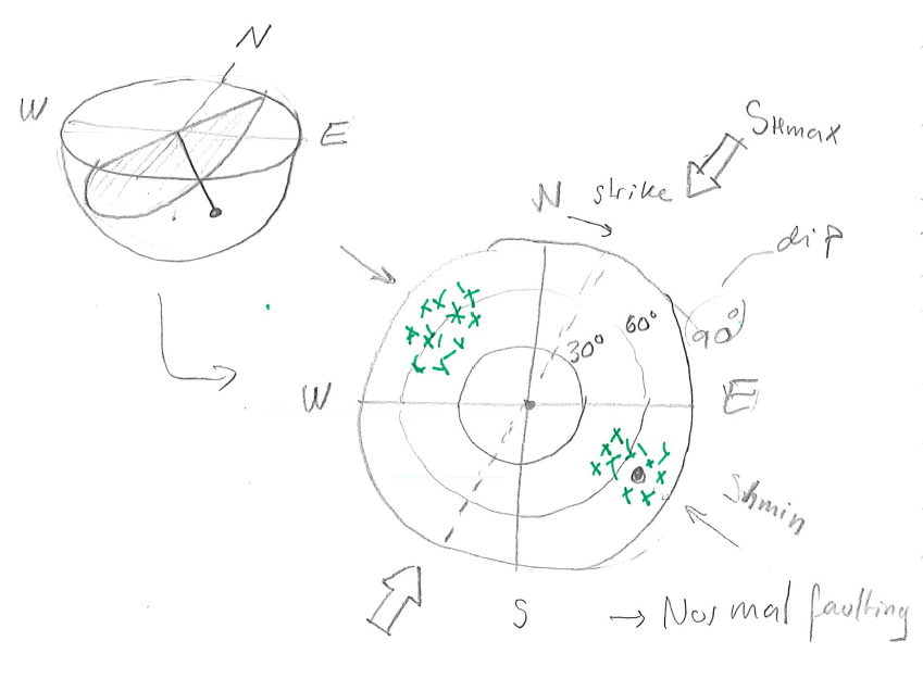
Stereonets are very useful for plotting the orientation of many faults in a single 2D plot 5.8. The stereonet represents a fault plane by a dot, which is the intersection of a line normal to the fault plane and a lower hemisphere projection. Visit this website for an online animation of stereonets: https://app.visiblegeology.com/stereonetApp.html.

Figure 5.8: Example of stereonet for mapping faults caused by a normal faulting stress regime. The crosses indicate faults at a strike around 030$^{\circ }$ with dips around 60$^{\circ }$SE and 60$^{\circ }$NW.

5.2.3 Faults in geological maps

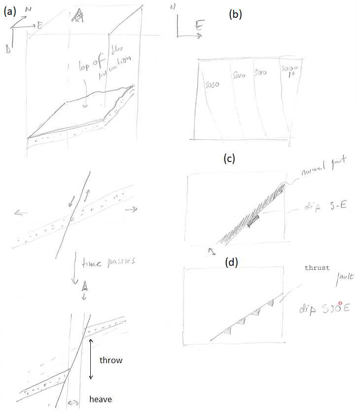
The geological map of a single formation, say a sandy layer formation, plots the top of such formation with depth in contour lines (Fig. 5.9b). Faults can also be represented in geological maps. Normal faults are represented as thick lines with thickness proportional to the heave of the fault (Fig. 5.9c). Reverse and thrust faults (negative heave) are plotted as lines with intermittent triangles on the dipping side (Fig. 5.9d).

Figure 5.9: Block representation and equivalent geologic map of sedimentary strata and faults.

Strike and dip of sedimentary strata can be reported in geological maps as shown in Fig. 5.10.

Figure 5.10: Strike and dip in geological maps.