Determination of horizontal stresses assuming limit equilibrium

Tectonic plates drive movements of the Earth's crust (Fig. 5.25). High temperatures and high effective stresses at great depth favor ductile deformation. Low temperatures and low effective stresses in the near-surface favor brittle failure.

Figure 5.25: Schematic of a section of the Earth's crust with brittle failure near surface and ductile deformation at depths greater than $\sim$ 16 km.

As a result of ubiquitous shear failure and faulting of the Earth's shallow crust, friction equilibrium limits the maximum magnitude of stresses imparted by tectonic strains. The limit is proportional to the frictional strength of faults. Because faults are cohesion-less, the frictional strength equation is simply:

$$\sigma_1 = q \sigma_3$$ (5.14)

(like sand, zero-intercept in the y-axis) where $\sigma _1$ is the maximum effective principal stress, $\sigma _3$ is the minimum effective principal stress, and $q=[1+\sin(\varphi)]/[1-\sin(\varphi)]$ is the anisotropy factor. The shear strength of the brittle crust has a direct implication in determining the maximum and minimum values of horizontal stresses for each stress regime. Frictional equilibrium of the brittle crust implies that horizontal stresses are controlled by shear failure. Hence, for

• normal stress regime (NF): $\sigma_{hmin}$ cannot be smaller than $\sigma_{v}/q$, for
• strike-slip stress regime (SS): $\sigma_{Hmax}$ cannot be greater than $q \: \sigma_{hmin}$, and for
• reverse stress regime (RF): $\sigma_{Hmax}$ cannot be greater than $q \: \sigma_{v}$.

As a result, the assumption of limit frictional equilibrium permits estimating minimum and maximum horizontal stresses if effective stresses $\sigma_{hmin}$ or $\sigma_{v}$ are known.

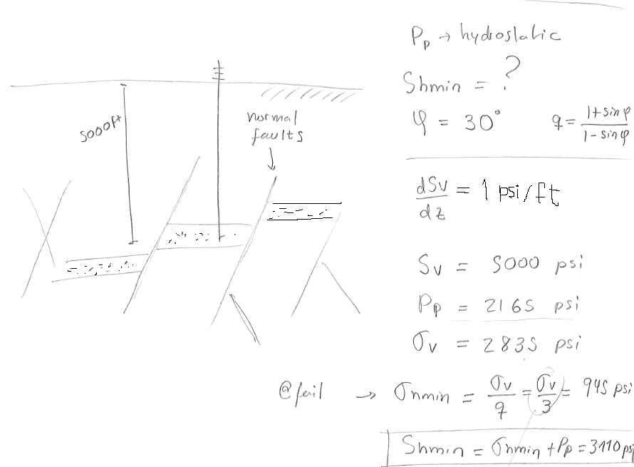
PROBLEM 5.13: A given site onshore is known to be subjected to a NF stress regime and hydrostatic pore pressure. Calculate the total horizontal minimum stress $S_{hmin}$ at a depth of 5000 ft assuming frictional equilibrium of faults and friction angle $\phi = 30^{\circ}$.

SOLUTION
The solution is a lower bound estimation of $S_{hmin}$ for normal faulting stress regime dictated by frictional equilibrium.

$\: \: \blacksquare$

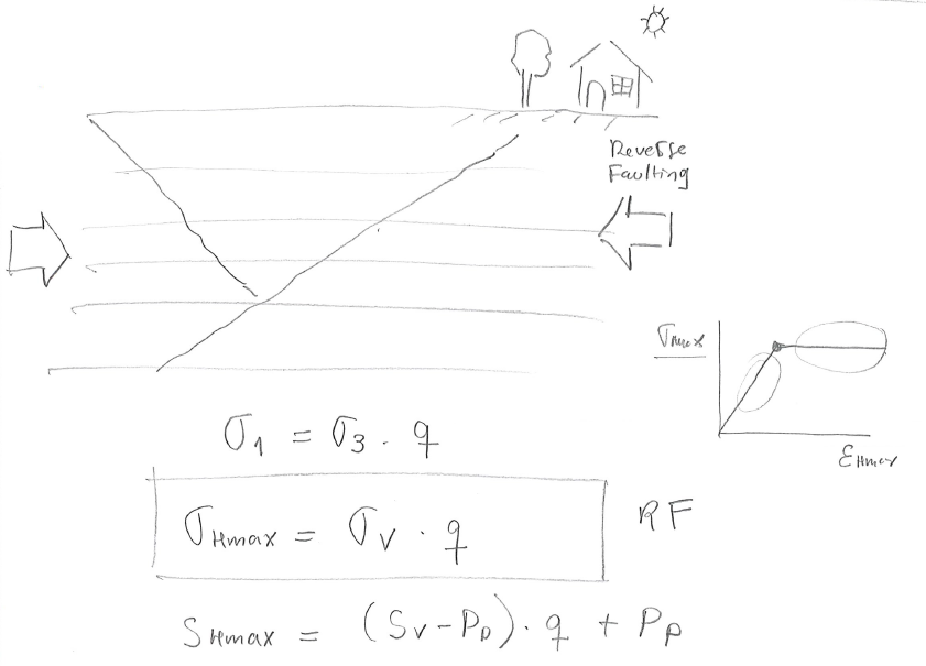
PROBLEM 5.14: A given site onshore is known to be subjected to a RF stress regime. Hard pressure is detected at 2000 ft with $\lambda_p=0.82$. Calculate the total maximum horizontal stress $S_{Hmax}$ at this depth assuming frictional equilibrium of faults and friction angle $\phi = 30^{\circ}$.

SOLUTION
The solution is an upper bound for $S_{Hmax}$.

Let us assume a lithostatic stress gradient of 1 psi/ft, hence

$$S_v = 1$$    psi/ft$$\times 2000$$    ft$$= 2000$$    psi$$$$

$S_v$ is the minimum principal since the site is subjected to reverse faulting regime. Given the overpressure parameter, pore pressure is

$$P_p = \lambda_p S_v = 0.82 \times 2000$$    psi$$= 1640$$    psi$$$$

and effective vertical stress is

$$\sigma_v = S_v - P_p = 2000$$    psi$$- 1640$$    psi$$= 360$$    psi

Finally, the maximum effective horizontal stress depends on the vertical effective stress (reverse faulting regime), so that

$$\sigma_{Hmax} = q \: \sigma_v = \frac{1+\sin 30^{\circ}}{1-\sin 30^{\circ}} 360$$    psi$$= 1080$$    psi

and therefore

$$S_{Hmax} = \sigma_{Hmax} + P_p = 1080$$    psi$$+ 1640$$    psi$$= 2720$$    psi$$\: \: \blacksquare$$

The bounding limits of minimum and maximum horizontal stress for a given vertical stress and pore pressure can be plotted through Zoback's (effective) stress polygon (Fig. 5.26). The colored lines represent the bounds for normal faulting stress regime (NF), strike-slip faulting stress regime (SS), and reverse faulting stress regime (RF).

Figure 5.26: The limits of horizontal stresses based on frictional equilibrium can be conveniently plotted in a “stress polygon” plot.

Fig. 5.27 shows an example of where the state of stress would plot in the stress polygon for a place with a stress regime that fluctuates from NF to SS with depth.

Figure 5.27: Application example of the stress polygon. This particular place exhibits a hybrid stress regime NF and SS depending on depth and likely rock lithology.