7.2 Hydraulic fractures in well testing

Understanding of hydraulic fractures is important for several applications in petroleum and geosystems engineering, from drilling and completion to enhanced oil recovery. The following field tests involve hydraulic fracturing and are suitable for specific applications.

7.2.1 Leak-off test

The leak-off test is conducted to measure the fracture gradient required for setting maximum mud pressure for drilling. The test is conducted with drilling mud after cementing the casing of the previous section in an open-hole.

Figure 7.2: Ideal leak off test pressure response with $S_v > S_{Hmax} = S_{hmin}$.

Execution of the leak-off test involves the following events:

• Injection of drilling mud at a constant rate causes the pressure to increase up to a maximum that depends on the near-wellbore stresses and tensile strength of the rock (Fracture breakdown pressure FBP or $P_b$). A change of slope may occur before FBP indicating a change of cavity volume, known as leak-off point (LOP).
• After fracture initiation, the fracture propagates at a velocity dictated by the fluid injection rate at a characteristic fracture propagation pressure (FPP).
• Shut-in of the pumps causes the pressure to decrease quickly at the instantaneous shut-in pressure (ISIP). Further pressure decrease originates from fluid in the fracture leaking off to the rock until the fractures closes at the fracture closure pressure (FCP).

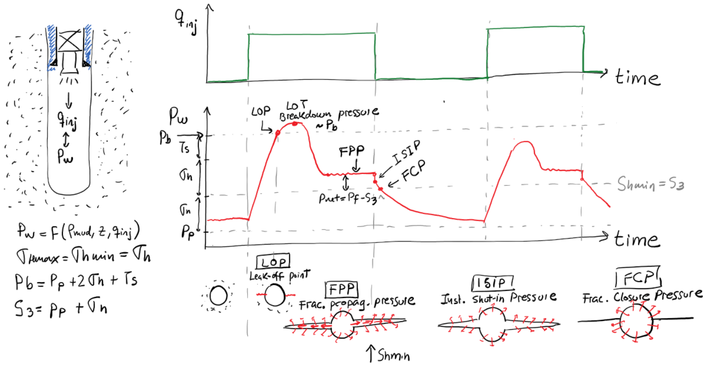
Figure 7.3 shows an example of a leak-off test using another notation for the leak-off point and breakdown pressure. Some studies suggest that a deviation from linearity at the beggining of the test indicates the opening of a small fracture (FIP) until it reaches a maximum pressure (UFP) after which it propagates at a rate faster than the injected fluid. An “extended” leak-off test requires to reach the UFP (or FPP) pressure. Sometimes the leak-off tests may be stopped before UFP to avoid large fractures in the well.

Figure 7.3: Example of real leak-off test data from an off-shore well. The pressure data show surface pressure readings.

7.2.1.1 Determination of the instantaneous shut-in pressure (ISIP)

The shut-in pressure is the maximum pressure before the pressure signature exhibits a gradual decay as a function of time due to shutting the pumps.

Figure 7.4: Example of determination of the instantaneous shut-in pressure from a fracture test.

7.2.1.2 Determination of the fracture closure pressure (FCP)

While the fracture is still open in an uncased borehole, fluids in the fracture leak off from both the wellbore and the fracture. Large leak-off surface (fracture walls and well) causes a rapid pressure decrease approximately proportional to the $\sqrt {t_{si}}$ (where $t_{si}$ is the time after shut-in). The pressure decrease rate slows down once the fracture closes (leak-off just from well) and departs from the $P$ vs. $\sqrt {t_{si}}$ linear trend. The fracture closure pressure (FCP) is the pressure at which this change in leak-off regime occurs (See example in Fig. 7.5). Fracture closure is interpreted to be approximately equal to the minimum principal total stress $S_3$.

Figure 7.5: Example of determination of the fracture closure pressure. Departure from the linear trend in a $P$ vs. $\sqrt {t_{si}}$ plot indicates fracture closure.

7.2.2 Diagnostic fracture initiation test (DFIT)

The objectives of the DFIT test are to determine permeability, determine pore pressure, and determine minimum principal stress $S_3$. The DFIT test is usually done in tight low-permeability reservoirs for completion purposes before a large hydraulic fracture treatment. The test involves small wellbore intervals using relatively small fracturing fluid injection volumes $\leqslant 10$ bbl. The injection rates are also relatively small ranging from $\sim$0.1 to 3 bbl/min. The DFIT test may be performed through perforations in already cased boreholes.

Figure 7.6: The DFIT test is performed with small injection volumes before actual hydraulic fracture completion.

The mechanics of the DFIT test is similar to the one of the leak-off test. The determination of FCP is similar to that of the leak-off test. More advanced methods use a “G-function” to determine FCP. The G-function is a dimensionless time function designed to linearize the pressure signal during normal fluid leak-off from a bi-wing fracture.

Figure 7.7: DFIT tests often utilize a “G-function” to determine the closure pressure. This method is based on the analysis of leak-off similar to the square-root-of-time method.

7.2.3 Step-rate test

The step rate test helps determine the maximum injection pressure in a wellbore designed for constant and long-term injection. Examples of injected fluids include water (liquid or vapor), CO$_2$, N$_2$, polymer mixtures, foam, natural gas, and produced water, among others. The objective is to determine the maximum injection pressure known as “formation parting pressure”.

The Procedure of the step-rate test is the following (See Figure 7.8):

1. Isolate the injection zone.
2. Inject fluid at successively higher injection rates during equal periods of time. Suggested schedule:
   • STEP TIME: 60 min if k$<$5md and 15-30 min if k$>$10 md
   • INJECTION RATE: 5, 10, 20, 40, 60, 80, 100% of maximum expected injection rate
3. Plot maximum stabilized pressure $P$ for each step as a function of injection rate $q$
4. The formation parting pressure is identified by the change in slope of $P$ vs. $q$

Figure 7.8: Schematic procedure of an ideal step-rate test. FPR: fracture propagation rate. FPP: fracture propagation pressure. Modified from [SPE 169513]

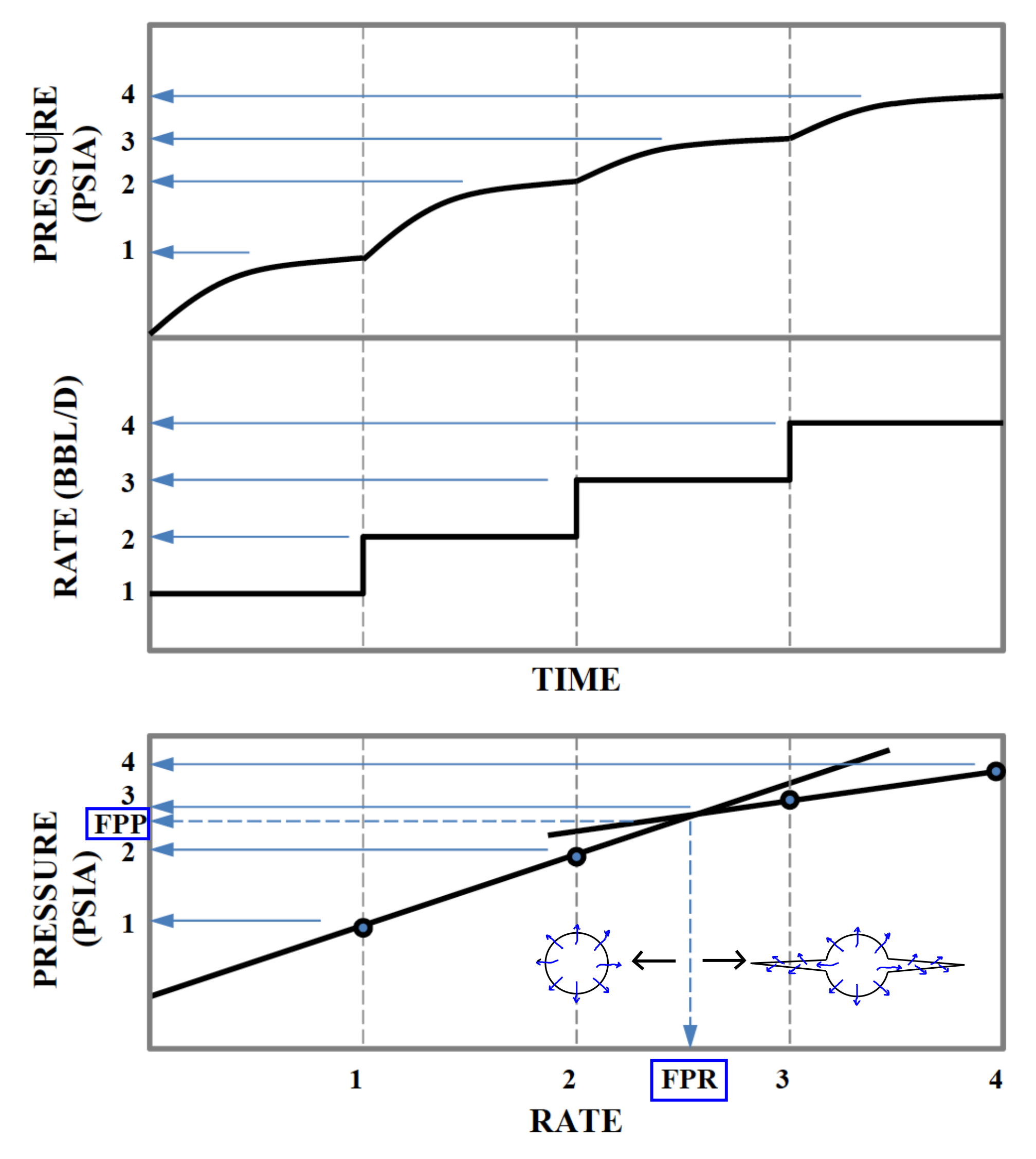Each injection step is performed until the pressure signal approaches an asymptotic response (top and middle figures). This maximum pressure $P$ at each step is then plotted as a function of injection rate $q$. The change in slope in the $P$ vs. $q$ plot (bottom) determines the formation parting pressure (FPP) and the formation parting rate (FPR). The change of slope occurs due to fracturing of the injector and can be interpreted as a change of the skin factor $s$ ($s>1$ means damage and $s<1$ means stimulation) in the wellbore equation

$$q = \frac{2 \pi h k} {\mu} \frac{P_e - P_w}{\ln (\frac{r_e}{r_w})+s}$$ (7.1)

Figure 7.9 shows an example of a step rate test conducted with steam. The step-rate test is required test by some regulatory agencies in order to safely dispose produced water. The objective is to avoid fracturing of the injector. There are ongoing efforts to regulate injection of large volumes that may not fracture the injector but could reactivate neighboring faults.

Figure 7.9: Example of actual injection-rate test for steam injection in an off-shore reservoir in California [data from SPE 169513].

Unintentional fracturing of the injector can be detrimental to sweep efficiency in EOR and IOR processes if the fracture connects the injectors and producers. On the other hand, fractures can be beneficial for sweep efficiency if oriented perpendicular to the direction of sweep (Fig. 7.10).

Figure 7.10: Example of fracturing in water-flooding with detrimental (left) and beneficial (right) implications for sweep efficiency. Circle plus arrow : injector, circle: producer, HF: hydraulic fracture.