5.5 Applications

5.5.1 Critically stressed fractures and permeability

The previous section shows how to calculate the normal effective stress $\sigma_n$ and shear stress $\tau$ components on an arbitrary oriented plane given the in-situ state of stress. A critically-stressed fracture (or fault) has shear stress and normal effective stress components with a ratio $\tau /\sigma _n$ which approaches the friction coefficient $\mu \sim$ 0.6-1.0. The fracture is said to be “critically stressed” because it is practically failing in shear. Such fractures -if they exhibit dilation during sliding- tend to be more hydraulically conductive than fractures with low $\tau /\sigma _n$ ratio (on the right of the Mohr circle and far left close to $\sigma _3$ - Fig. 5.26). Natural fractures can help fluid drainage. Traditionally, fracture permeability has been thought to be dependent on effective normal stress only $k_{frac} = f(\sigma_n)$. The concept of critically stressed fractures adds one more level of dependency to fracture permeability such that it is also a function of shear stress $k_{frac} = f(\sigma_n,\tau)$.

Figure 5.24: Fractures with a ratio $\tau /\sigma _n \sim \mu$ in brittle rocks tend to have higher permeability than other fractures with $\tau /\sigma _n \rightarrow 0$ and induce permeability anisotropy in fractured rock masses.

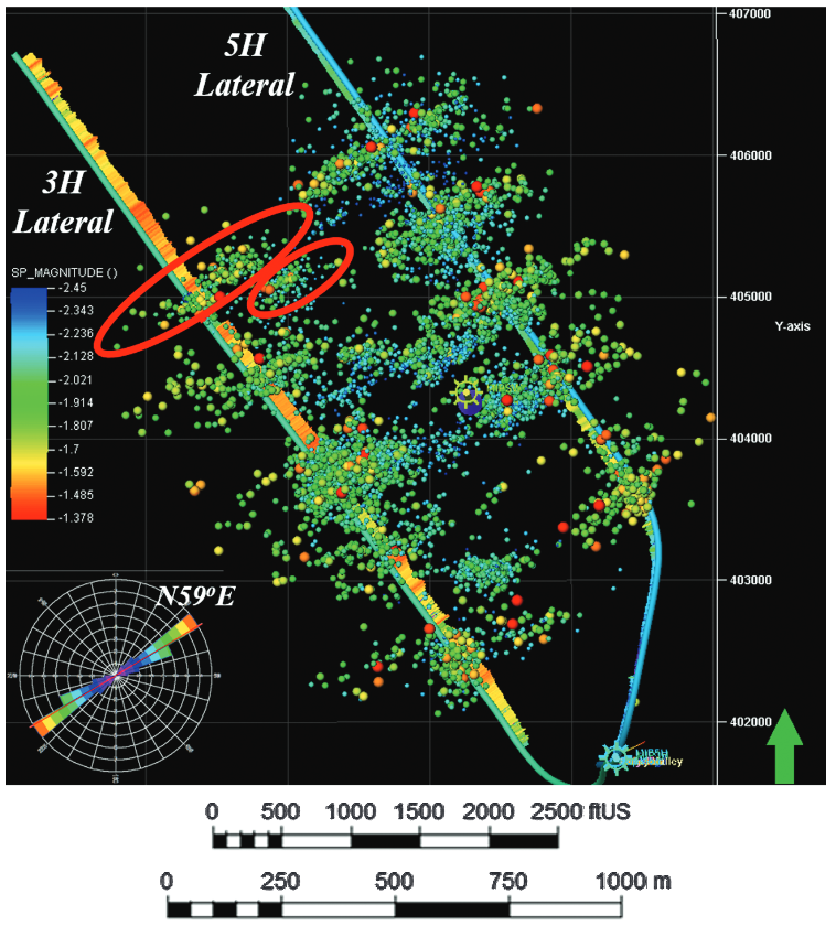
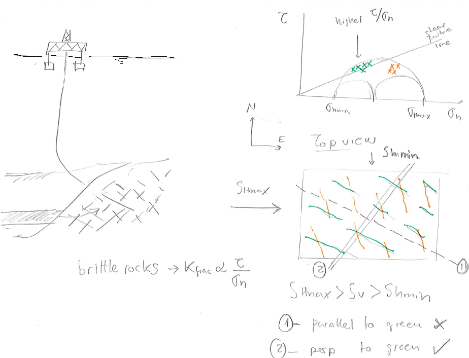
If critically oriented fractures have higher permeability than non-critically oriented fractures, then, the state of stress determines which fractures are hydraulically conductive and also determines permeability anisotropy in a fractured reservoir. Fractures that have an orientation that favors high $\tau /\sigma _n$ ratio are said to be “critically oriented” 5.26. This dependence is particularly important in unconventional formations where fracture permeability plays a critical role in determining production rates. The orientation of such fractures is critical for determining the orientation of a horizontal wellbore that minimizes the least resistance path of fluids from the rock matrix to the wellbore.

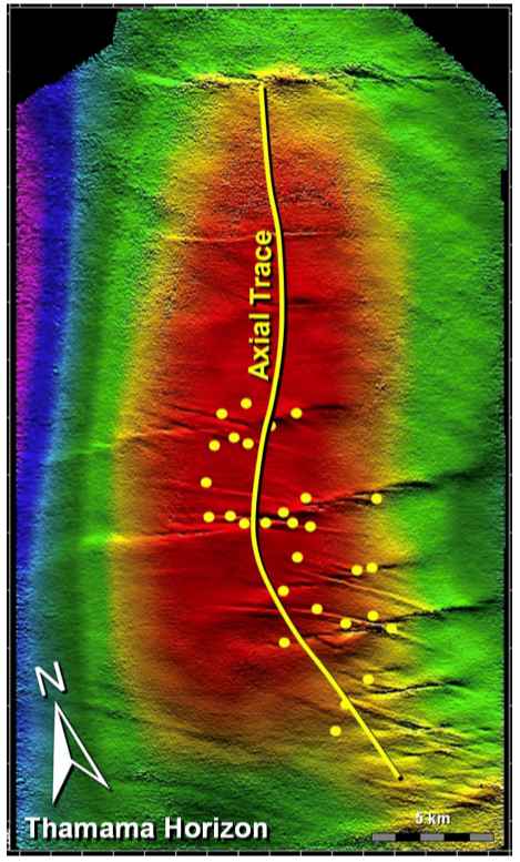
Fractures can also create and reactivate during hydraulic fracturing. The dots in Fig. 5.25 indicate micro-to-nano earthquakes hypocenters (at depth) triggered by rock failure during hydraulic fracturing. Hydraulic fracturing imparts changes of stresses that reactivate some critically oriented fractures in tight reservoirs. These reactivated fractures are useful to contribute to increase the permeability of tight reservoirs at the large scale (also known as Stimulated Reservoir Volume SRV). Some of these created fractures may close and seal-off fairly quickly upon depletion if not propped. Significant ongoing research addresses how to maintain the permeability of these fractures in the long-term.

Figure 5.25: Shear fracture reactivation in multistage hydraulic fracturing evidenced by microseismic activity - Image from [Wilson et al. 2018 - Interpretation]

Figure 5.26: Example of horizontal wellbore placement in a fractured reservoir. The horizontal wellbore should be ideally perpendicular to critically stressed fractures to take advantage of their high permeability.

The same reasoning applies to large faults. There are faults that may be more easily reactivated due to pore pressure changes because of their orientation with respect to the current state of stress (See subsection 5.5.4).

5.5.2 Determination of horizontal stresses assuming limit equilibrium

Tectonic plates drive movements of the Earth's crust (Fig. 5.27). High temperatures and high effective stresses at great depth favor ductile deformation. Low temperatures and low effective stresses in the near-surface favor brittle failure.

Figure 5.27: Schematic of a section of the Earth's crust with brittle failure near surface and ductile deformation at depths greater than $\sim$ 16 km.

As a result of tectonic movement, there is ubiquitous shear failure and faulting of the Earth's shallow crust. The frictional strength of faults limits the maximum magnitude of stresses imparted by tectonic strains (Figure 5.28). Hence, horizontal stresses are proportional to tectonic strains in the elastic region, but their maximum value is limited by fault strength.

Figure 5.28: Schematic of in-situ stress as a function of tectonic strains $\varepsilon _{tect}$ and failure strength. The frictional strength of faults controls stress once the elastic region is exceeded.

Because faults are cohesion-less, the frictional strength equation is simply:

$$\sigma_1 = q \: \sigma_3$$ (5.16)

(like sand, zero-intercept in the y-axis) where $\sigma _1$ is the maximum effective principal stress, $\sigma _3$ is the minimum effective principal stress, and $q=[1+\sin(\varphi)]/[1-\sin(\varphi)]$ is the anisotropy factor.

The shear strength of the brittle crust has a direct implication in determining the maximum and minimum values of horizontal stresses for each stress regime once the tectonic strains are surpassed. Frictional equilibrium of the brittle crust implies that minimum and maximum attainable values of horizontal stresses are controlled by shear failure. Hence, for

• normal stress regime (NF): $\sigma_{hmin}$ cannot be smaller than $\sigma_{v}/q$, for
• strike-slip stress regime (SS): $\sigma_{Hmax}$ cannot be greater than $q \: \sigma_{hmin}$, and for
• reverse stress regime (RF): $\sigma_{Hmax}$ cannot be greater than $q \: \sigma_{v}$.

As a result, the assumption of limit frictional equilibrium permits estimating minimum and maximum horizontal stresses if effective stresses $\sigma_{hmin}$ or $\sigma_{v}$ are known.

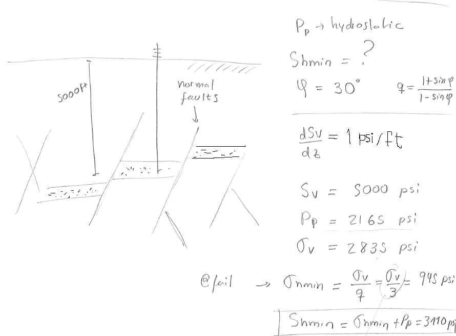
PROBLEM 5.13: A given site onshore is known to be subjected to a NF stress regime and hydrostatic pore pressure. Calculate the total horizontal minimum stress $S_{hmin}$ at a depth of 5,000 ft assuming frictional equilibrium of faults and friction angle $\varphi = 30^{\circ}$.

SOLUTION
The solution is a lower bound estimation of $S_{hmin}$ for normal faulting stress regime dictated by frictional equilibrium.

$\: \: \blacksquare$

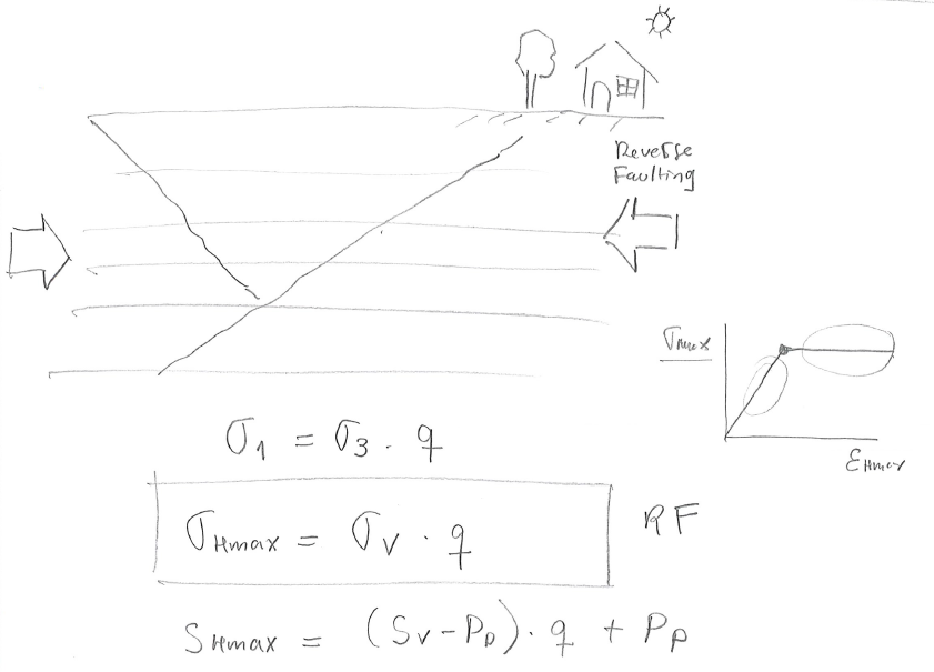
PROBLEM 5.14: A given site onshore is known to be subjected to a RF stress regime. Hard pressure is detected at 2,000 ft with $\lambda_p=0.82$. Calculate the total maximum horizontal stress $S_{Hmax}$ at this depth assuming frictional equilibrium of faults and friction angle $\varphi = 30^{\circ}$.

SOLUTION
The solution is an upper bound for $S_{Hmax}$.

Let us assume a lithostatic stress gradient of 1 psi/ft, hence

$$S_v = 1$$    psi/ft$$\times 2000$$    ft$$= 2000$$    psi$$$$

$S_v$ is the minimum principal since the site is subjected to reverse faulting regime. Given the overpressure parameter, pore pressure is

$$P_p = \lambda_p S_v = 0.82 \times 2000$$    psi$$= 1640$$    psi$$$$

and effective vertical stress is

$$\sigma_v = S_v - P_p = 2000$$    psi$$- 1640$$    psi$$= 360$$    psi

Finally, the maximum effective horizontal stress depends on the vertical effective stress (reverse faulting regime), so that

$$\sigma_{Hmax} = q \: \sigma_v = \frac{1+\sin 30^{\circ}}{1-\sin 30^{\circ}} 360$$    psi$$= 1080$$    psi

and therefore

$$S_{Hmax} = \sigma_{Hmax} + P_p = 1080$$    psi$$+ 1640$$    psi$$= 2720$$    psi$$\: \: \blacksquare$$

The bounding limits of minimum and maximum horizontal stress for a given vertical stress and pore pressure can be plotted through Zoback's (effective) stress polygon (Fig. 5.29). The colored lines represent the bounds for normal faulting stress regime (NF), strike-slip faulting stress regime (SS), and reverse faulting stress regime (RF).

Figure 5.29: The limits of horizontal stresses based on frictional equilibrium can be conveniently plotted in a “stress polygon” plot.

For example, the state of stress for a place with a stress regime that fluctuates from NF to SS with depth would plot at the intersection of NF and SS lines in the stress polygon (Fig. 5.30).

Figure 5.30: Application example of the stress polygon. This particular place exhibits a hybrid stress regime NF and SS depending on depth and likely rock lithology.

5.5.3 Determination of stress regime and horizontal stress direction from fault orientation

Mapping of faults and fractures in the subsurface helps interpret the state of stress that caused such fractures. In some cases the state of stress that caused such faults may be still acting today. The example in Fig. 5.31 shows an example of strike-slip conjugate faults. The maximum horizontal stress that caused these shear faults was aligned with the bisectrix of the two fault strikes, about E10$^{\circ }$S.

Figure 5.31: Seismic image of the top of an anticline structure (red: shallower, blue: deeper, TOP VIEW). The discontinuities in the seismic image are strike-slip faults. Image from [IPTC-10646-MS].

5.5.4 Fault reactivation

Depletion and injection of fluids in the subsurface cause changes in pore pressure and therefore on effective stresses. Fluid injection such as in hydraulic fracturing, water-flooding, and waste-water disposal can reach adjacent faults (if any) and decrease the effective normal stress $\sigma_n = S_n - P_p$ acting on faults. In hydraulic fracturing, the injection of fluids is temporary and limited to the fracture completion size. In water-flooding, pressure build-up is limited by the producer wells. In waste-water injection, the pressure build-up is controlled by the aquifer size, compressibility and compartmentalization.

Figure 5.32: Fault reactivation. Injection of fluids changes the pore pressure and lowers effective normal stress on faults increasing $\tau /\sigma _n$.

The change of stresses produced by increases of pore pressure assuming constant total vertical stress and negligible poroelastic effects is

$$\left\lbrace \begin{array}{l} \Delta \sigma_v = - \Delta P_p \\ \Delta \sigma_{hmin} \leq - \Delta P_p \\ \end{array}\right.$$ (5.17)

The result is a shift of the Mohr circle to the left, closer to the shear failure or “reactivation” line. The magnitude of change of pore pressure needed to reactivate a fault is (at least) equal to the horizontal distance between the point of the Mohr-circle of such fault and the failure line. Hence, a critically oriented fracture needs the lowest $\Delta P_p$ to reactivate.

The reactivation of faults may result in induced seismicity. The imparted change of fault permeability depends on the fault filling, known as fault gouge. Both, induced seismicity and change in fault permeability depend on the failure properties of the fault gouge. Brittle failure results in high energy release through induced seismicity and increases of fault permeability, while ductile failure results in low energy release through seismicity and decreases or minor increases of permeability. An undesired consequence of fault reactivation is the loss of hydrocarbon trapping ability at fault structural traps (e.g., https://www.youtube.com/watch?v=OtJTI4nv1QI). Figure 5.33 shows an example of induced seismicity with magnitude $M<2$ in the Richter scale due to injection of carbon dioxide in the Mount Simon Sandstone. The seismicity originates mostly from reactivation of faults below the reservoir formation in basement formations. The regional stress regime alternates between strike-slip and reverse (See Figure 2.24).

Figure 5.33: Fault reactivation observed through microseismicity due to CO$_2$ injection in a sandstone formation [Bauer et al, 2016 - IJGGC]. Notice the alignment of events that likely reveals fault strike. Significant microseismicity occurs as far as 0.6 miles away from the injector.