4.3 Shear failure

4.3.1 Frictional Strength

The shear strength of rocks depends on the cohesive strength of the rock $S_0$ (to be explained later) and the internal frictional strength of the rock. The frictional strength depends on friction forces, where the force $F_T$ needed to displace an object resting on a surface depends on the friction coefficient $\mu$ and applied normal force $F_N$, such that $F_T = \mu F_N$ (Figure 4.8). Hence, if the normal force $F_N=0$, then $F_T = 0$. The frictional force $F_T$ increases linearly with the value of the normal force $F_N$.

Figure 4.8: Friction forces and the friction coefficient. (a,b) Frictional force required to move a solid box. (c) Extension to granular media.

Similarly, uncemented sediments can resist shear stresses with the application of an effective “confining” compressive stress (remember the example of the vacuum-sealed coffee). The maximum shear stress $\tau$ in uncemented sands is proportional to the normal effective stress $\sigma_n$ through an “internal” friction coefficient $\mu_i$ (red line in Figure 4.9). The sand is at shear failure when the shear line $\tau = \mu_i \sigma_n$ intercects the state of stress represented by the Mohr circle (Check this online Mohr's circle drawer).

Figure 4.9: Frictional strength of uncemented sediments.

The Mohr circle represents all possible state of stresses depending on the plane at which you measure $\sigma_n$ and $\tau$. Notice that from all those possible state of stresses, there is just one state of stress that intersects the line $\tau = \mu_i \sigma_n$. That plane is the plane at which a shear fracture would form. Similarly to Figure 4.8, if $\sigma_n = 0$ then $\tau = 0$, so the sand has no strength whatsoever without an effective compressive stress. The friction coefficient $\mu_i$ is often expressed as a friction angle $\varphi$, where $\tan (\varphi) = \mu_i$. Typical values of $\mu_i$ vary from 0.4 to 1.0. For example, if $\mu_i=0.5$, then $\varphi \sim 30^{\circ}$.

4.3.2 Unconfined compression strength

Cemented rocks can bear shear stresses with zero effective lateral stress $\sigma_r = 0$ ($\sigma _r$ for radial effective stress as in cylindrical samples). Figure 4.10 shows an unconfined cylindrical rock loaded (on the top face) to failure with a compression effective stress $\sigma_a$. We call $UCS$ (Unconfined Compression Strength) to the maximum compression stress (applied in axial direction) the rock can hold under unconfined conditions. Axisymmetric tests require rocks samples in which the length should be about twice the diameter to minimize shear end-effects (as in short samples) and buckling instabilities (as in long samples).

Figure 4.10: Unconfined compression strength: schematic diagram, stress-strain plot and corresponding Mohr circle.

4.3.3 Confined strength: the triaxial test

Let us now apply an effective compressive “confining” stress $\sigma_r \neq 0$ (Figure 4.11). The measured peak stress is higher than the peak stress without confining stress. The increment in peak stress will be a function of the internal frictional strength of the rock. Hence, the maximum shear stress $\tau$ will be a function of both the rock cohesive strength $S_0$ and the applied normal effective compressive stress $\sigma_n$ through the Coulomb failure criterion expressed in the following equation:

$$\tau = S_0 + \mu_i \sigma_n$$ (4.2)

Figure 4.11: Shear strength: Coulomb failure criterion. The cylindrical rock sample bears a radial confining stress $\sigma _r$.

With a linear shear failure criterion, a fracture will ideally form at an angle $\pi/4 + \varphi/2$ from the plane where the maximum principal stress is applied. Such plane will also be co-linear with the intermediate principal stress. For a typical value of $\varphi \sim 30^{\circ}$, $\pi/4 + \varphi/2 = 60^{\circ}$.

PROBLEM 4.2: In the following uncemented sediment sample and corresponding figure:
a) Which is the point in the Mohr circle with maximum $\tau /\sigma _n$?
b) What is the angle of the failure plane?
c) What is the ratio $\sigma_a / \sigma_r$ at failure?

SOLUTION
a) The point in the Mohr circle with maximum ratio $\tau /\sigma _n$ is the one that touches the yield line, for which $\tau / \sigma_n = \mu_i$

b) Let us use the figure above to solve the problem. The top side of the sample is subjected to stress $(\sigma_a,0)$ in the $\sigma_n$-$\tau$ plane. The lateral side of the sample is subjected to stress $(\sigma_r,0)$ in the $\sigma_n$-$\tau$ plane. The state of stress $(\sigma_n,\tau)$ at failure can be located going $\pi/2 + \varphi$ counterclockwise from $(\sigma_a,0)$ to $(\sigma_r,0)$. The plane of shear failure corresponds to this point and it is at $(\pi/2 + \varphi)/2$ from the top side towards the lateral side. Notice that going from $(\sigma_a,0)$ to $(\sigma_r,0)$ takes 180 $^{\circ} = \pi/2$ in the Mohr circle.

c) Let us use $C$ (center of the circle) and $R$ (radius of the circle) to express $\sigma_a / \sigma_r$:

$$\frac{\sigma_a}{\sigma_r} = \frac{C + R}{C-R} = \frac{C+C \sin ... ...-C \sin \varphi} = \frac{1+\sin \varphi}{1-\sin \varphi} \: \: \blacksquare$$

Sometimes, it is easier to think (and compute) shear failure parameters based on principal stresses rather than on normal and shear stress (Figure 4.12). Coulomb's failure criterion (Eq. 4.2) can be written as

$$\sigma_1 = UCS + q \: \sigma_3$$ (4.3)

where $\sigma _1$ is the effective maximum principal stress at failure, $\sigma _3$ is the effective minimum principal stress and $q$ is the friction parameter function of the friction angle (warning: this is not the same $q$ from the $p'-q$ or $\sigma_m-q$ space). It can be shown that,

$$q = \frac{1 + \sin \varphi}{1 - \sin \varphi}$$ (4.4)

For a typical $\varphi ~ 30^{\circ}$, $q = 3$. The friction coefficient can be calculated from the friction parameter $q$ with the following equation:

$$\mu_i = \frac{q-1}{2 \sqrt{q}}$$ (4.5)

$UCS$ can also be expressed in terms of cohesive strength as

$$UCS = 2 S_0 \left( \frac{1 + \sin \varphi}{1 - \sin \varphi} \right)^{1/2} = 2 S_0 \sqrt{q}$$ (4.6)

Figure 4.12: Equivalency of the Coulomb criterion in terms of shear and normal stresses and in terms of principal stresses.

Figure 4.13 summarizes shear strength properties for various cemented rocks.

Figure 4.13: Average values of cohesive strength and internal friction angle for various types of rocks (original data from [Zoback, 2013]).

4.3.4 Triaxial tests of fluid saturated rocks and sediments

The shear strength of rocks depends on effective stresses, not on total stresses. In the field and the laboratory, however, we usually measure total stresses $(S_1,S_2,S_3)$ instead of effective stresses $(\sigma_1,\sigma_2,\sigma_3)$. The shear strength of rocks is measured in a triaxial frame (Fig. 4.15-a). A cylindrical (axisymmetric) triaxial frame can apply independently a confining pressure (that converts into stress) $P_c$, a deviatoric stress $\sigma_D$, and a pore pressure $P_p$.

The confining stress is applied by means of a deformable sleeve around the rock by changing the confining fluid pressure $P_c$ with a fluid pump. The confining fluid is usually hydraulic oil or water. The sleeve makes it possible to apply an effective confining stress and prevents confining fluid to enter into the rock pores and mix with the pore fluid. The confining pressure is maintained constant in a typical deviatoric triaxial test $P_c = cst$.

The pore fluid pressure $P_p$ is applied with another fluid pump. A fluid conduit connects the pump with the rock pore space. Some triaxial frames have two pore fluid outlets to measure permeability during loading. Notice that $P_p < P_c$, otherwise the sleeve would inflate like a balloon inside the pressure vessel. The pore pressure is maintained constant in a typical deviatoric triaxial test $P_p = cst$.

The deviatoric stress $\sigma_D$ is applied through axial loading with a piston that compresses the rock in axial direction. The deviatoric stress is defined as $\sigma_D =S_1 - S_3$, where $S_1$ is the total maximum stress applied with the frame and $S_3$ is the minimum total stress (equal to the confining pressure $S_3 = P_c$) (Figure 4.14). Notice that in a cylindrical triaxial frame $S_2=S_3$ and $S_1 - S_3=\sigma_1-\sigma_3$. The deviatoric stress is increased with a constant displacement (strain) rate $d \varepsilon_a / dt = cst$ in a typical deviatoric triaxial test.

Figure 4.14: Schematic diagram of stresses and pressures in the axisymmetric triaxial test. $S_1$: total axial stress, $S_3$: total radial stress ($=P_c$: confining pressure), $P_p$: pore pressure.

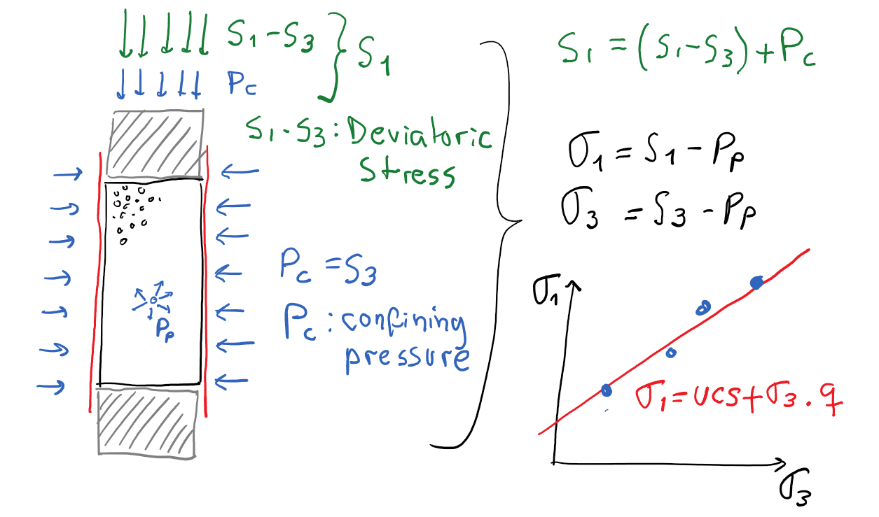The data shown in Fig. 4.15-b summarizes the results of 14 independent triaxial tests: $S_3$ is the confining pressure for each experiment, $S_1$ is the maximum stress measured at failure, and $P_p$ is the preset pore pressure. The data shows that the maximum principal stress $S_1$ (measured at failure) tends to increase as $S_3$ increases and tends to decrease as $P_p$ increases. When the data is corrected to effective stresses (Fig. 4.15-c), it becomes clear that there is just one relationship between $\sigma_1 = (S_1 - P_p)$ and $\sigma_3 = (S_3 - P_p)$.

The equation that links these two quantities is Eq. 4.12. It is usually easier to calculate $UCS$ and $q$ from fitting a straight line to $\sigma _1$ (failure)- $\sigma _3$ data, and then calculate cohesive strength from Eq. 4.6, friction angle as

$$\varphi = \arctan \left( \frac{q-1}{2\sqrt{q}} \right)$$ (4.7)

PROBLEM 4.3: Fit a line (manually) to the data shown in Fig. Fig. 4.15-c for the Darley Dale sandstone and calculate $UCS$, $q$, $S_0$, $\varphi$ and $\mu_i$.

SOLUTION
The red line in Fig. 4.15-c was manually drawn ignoring the point with the highest confining stress. Hence, this line is accurate only when $S_3 \leqslant 80$ MPa.

The red line hits the y-axis at $S_1 \sim 80$ MPa, hence,

$$UCS = 80$$    MPa$$$$

The parameter $q$ is the slope of the red line. Taking the entire line length:

$$q = \frac{\Delta \sigma_1}{\Delta \sigma_3} = \frac{520 \text{ MPa}}{110 \text{ MPa}} = 4.73$$

Finally, using Eqs. 4.6 and 4.7:

$$S_0 = \frac{UCS}{2 \sqrt{q}} = \frac{80 \text{MPa}}{2 \sqrt{4.73}} = 18.4 \text{MPa}$$

$$\varphi = \arctan \left( \frac{q-1}{2\sqrt{q}} \right) = \arctan \left( \frac{4.73-1}{2\sqrt{4.73}} \right) = 40.6^{\circ}$$

$$\mu_i = \tan (\varphi) = \tan (40.6^{\circ}) = 0.86 \: \: \blacksquare$$

In the process of triaxial loading, rocks begin by decreasing volume (compression loading) but may show positive changes of volumetric strain $\varepsilon_v = \varepsilon_a + 2\varepsilon_r$ approaching failure. That is, the rock may start shrinking but it may dilate close to failure giving $d \varepsilon_v/dt<0$ (dilation is negative). At this point the rock is not elastic anymore and develops damage inside. Considerable damage often starts at 50% to 70% of the peak stress.

Figure 4.15: Triaxial testing. (a) Axisymmetric triaxial frame comprising a pressure vessel, fluid pumps and a reaction frame to apply axial load (not visible in figure). (b) Example results of 14 independent triaxial tests on Darley Dale sandstone as a function of total stresses and pore pressure. (c) Data from -b replotted as effective stresses. Rocks failure is explained through effective stresses, not through total stresses.