5. Stresses on Faults and Fractures

5.1 Introduction

Changes of stresses in the subsurface lead to deformation of geological structures. Deformations can be grouped in (1) gradual and continuous, such as folding that creates an anticline, and (2) abrupt and discontinuous, such as faults. The creation of fault discontinuities depends on loading strain rate and rock properties including rock brittleness. Faults are the result of brittle rock failure in shear at the large scale (Fig. 102).

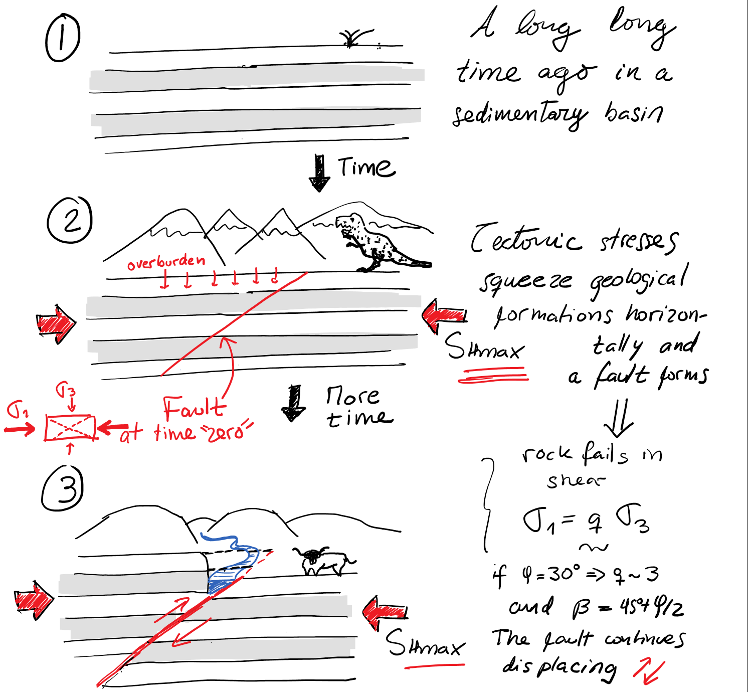
Fig. 102 Simplified schematic of the genesis of a thrust fault.

Faults usually cut through several sedimentary strata (See outcrop fault examples in Fig. 103). Faults are important in energy geomechanics because they limit the magnitude of horizontal stresses, may constitute structural traps for fluid flow, favor reservoir compartmentalization, and other times create high permeability conduits for fluid flow. A map of faults and rock units in Texas is available here.

Fig. 103 Examples of faults as seen in outcrops.

5.2 Mapping of faults and fractures

Faults in subsurface formations are usually mapped through seismic reconstruction (see example in Fig. 104) and wellbore imaging.

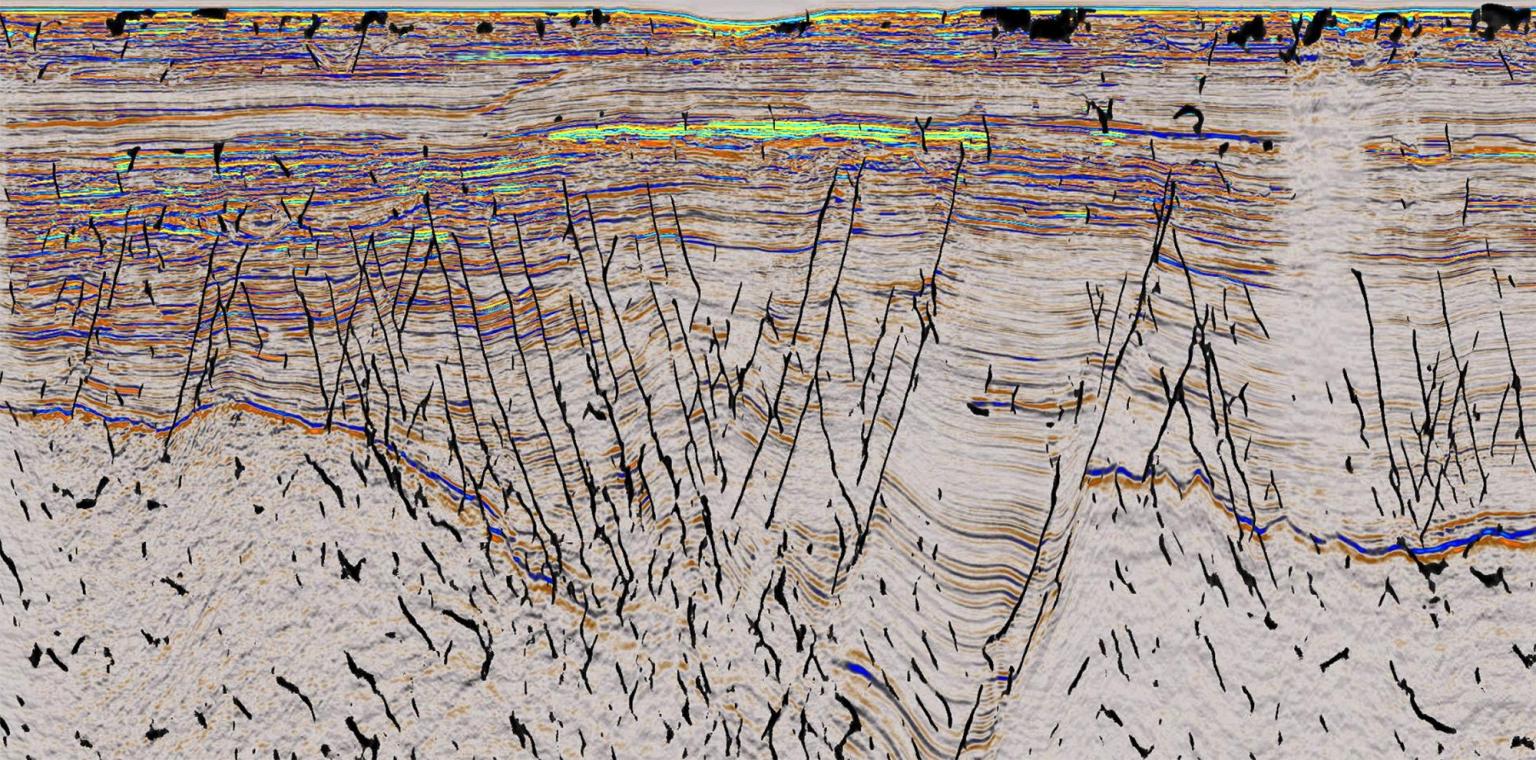
Fig. 104 Fracture mapping in seismic images (Credit: ConocoPhillips).

Fig. 105-a shows the typical signature of fractures in a wellbore. An anomaly of electrical resistivity or ultrasonic P-wave velocity facilitates recognizing the fracture (dark pixels in the image). The reconstruction of this image (Fig. 105-b) helps measure fracture orientation (strike and dip - Fig. 105-c).

Fig. 105 Fracture mapping in wellbores. \hl{[make your own]}

Comprehensive fracture mapping helps create 3D reservoir models that account for fault and fracture geomechanics (Fig. 106). The magnitude of shear and normal stresses on faults and fractures depends on their orientation respect to the in-situ stress tensor.

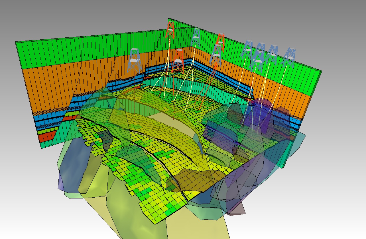
Fig. 106 Reservoir model example including faults (Courtesy Baker Hughes).

5.2.1 Orientation of planes with respect to the geographical coordinate system

Imagine any plane (such as the plane shown in Fig. 107) cutting horizontal sedimentary strata. The \textit{strike} is the line which results from the intersection of such plane and a horizontal plane. The magnitude of the strike is the angle between the strike line and the north. The angle of \textit{dip} is the angle between a horizontal plane and the plane under consideration. A layer is said to dip in a given direction when it gets deeper at the fastest rate into such direction. One can think of the \(dip\) as the direction of a droplet of water moving down on such plane.

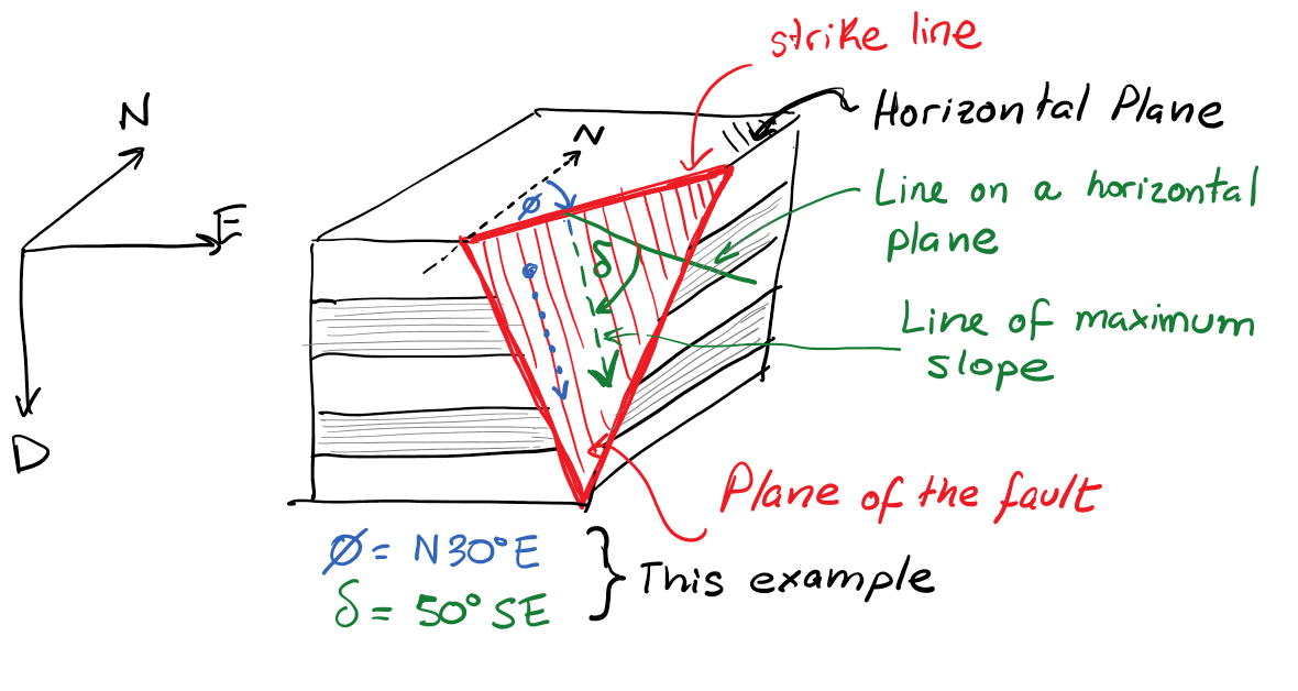
Fig. 107 Definition of strike and dip. \hl{[make vectorial plot]}

There are two conventions for reporting the magnitude of strike.

• Quadrant convention: it reports strike with angles ranging from 0 to 45\(^{\circ}\). The quadrant convention is useful in the field. For example:

  1. “N45\(^{\circ}\)E” means 45\(^{\circ}\) clockwise from the North towards the East

  2. “S45\(^{\circ}\)W” means 45\(^{\circ}\) clockwise from the South towards the West

  3. “N45\(^{\circ}\)E” is the same as “S45\(^{\circ}\)W” (Fig. 108)

• Azimuth convention: it reports strike with angles ranging from 0 to 360\(^{\circ}\) measured from the North to the strike “vector” in clockwise direction (see Fig. 129). The azimuth convention is most useful for data analytics and mathematical implementation. For example:

  1. “045\(^{\circ}\)” for a a fault strike N45\(^{\circ}\)E and dipping SE.

  2. “225\(^{\circ}\)” for a a fault strike N45\(^{\circ}\)E and dipping NW.

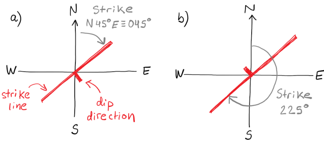
Fig. 108 Quadrant and azimuth terminology for strike. Notice that in the azimuth convention dip direction matters when defining the strike angle.

The dip is the angle between a horizontal plane and the line of maximum slope in the measured plane. It is reported with angles between 0 and 90\(^{\circ}\). The maximum dip is 90\(^{\circ}\) (vertical plane). If the layer/fault is tipped even further it is said to be overturned. The dip is usually accompanied by the direction in which the plane is dipping in quadrant notation. For example, the plane in Fig. 107 dips about 60\(^{\circ}\)SE, 60 degrees toward the South-East. This interactive map shows the strike and dip of major faults in Texas.

5.2.2 Stereonets for plotting fault orientation

Stereonets are very useful for plotting the orientation of many faults in a single 2D plot Fig. 109. The stereonet represents a fault plane by a dot, which is the intersection of a line normal to the fault plane and a lower hemisphere projection. Visit this website for an online animation of stereonets.

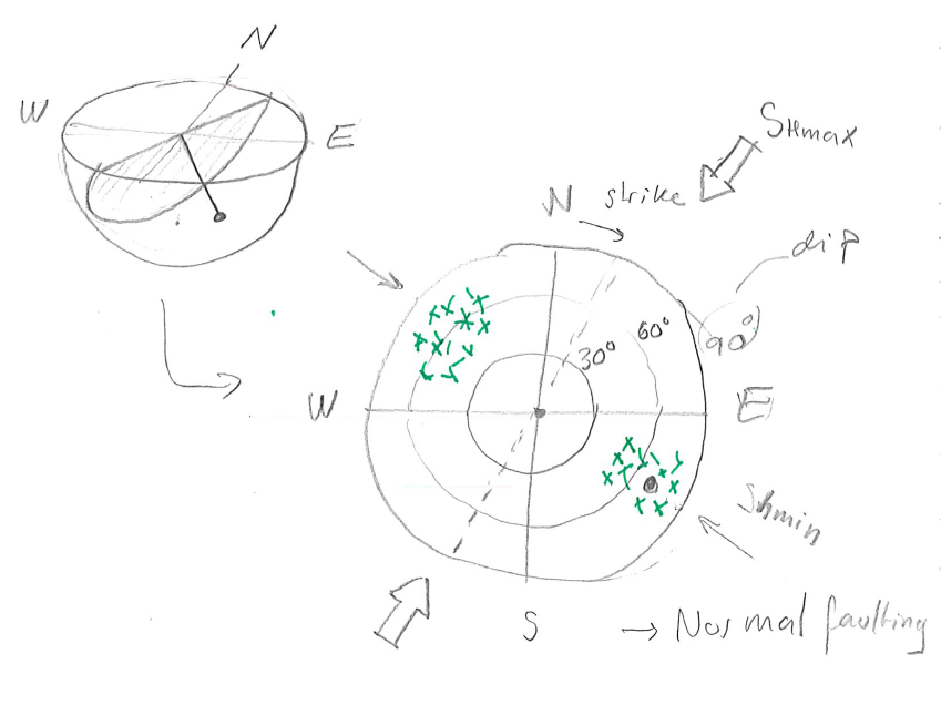
Fig. 109 Example of stereonet for mapping faults caused by a normal faulting stress regime. The crosses indicate faults at a strike around 030\(^{\circ}\) with dips around 60\(^{\circ}\)SE and 60\(^{\circ}\)NW.

5.2.3 Faults in geological maps

The geological map of a single formation, say a sandy layer formation, plots the top of such formation with depth in contour lines (Fig. 110-b). Faults can also be represented in geological maps. Normal faults are represented as thick lines with thickness proportional to the heave of the fault (Fig. 110-c). Reverse and thrust faults (negative heave) are plotted as lines with intermittent triangles on the dipping side (Fig. 110-d). Fig. 111 shows an example application of this convention to the North Sea.

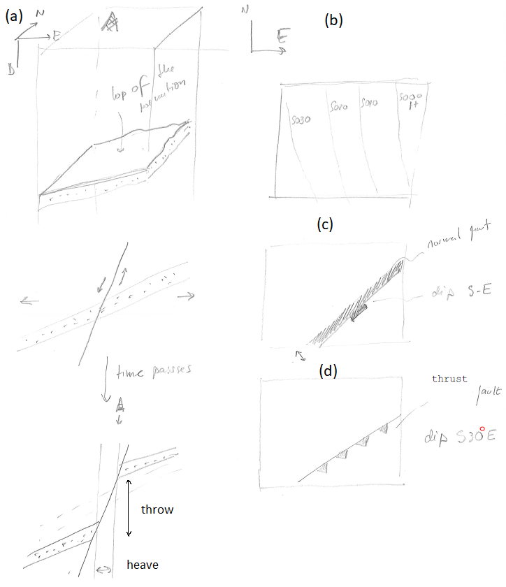
Fig. 110 Block representation and equivalent geologic map of sedimentary strata and faults.

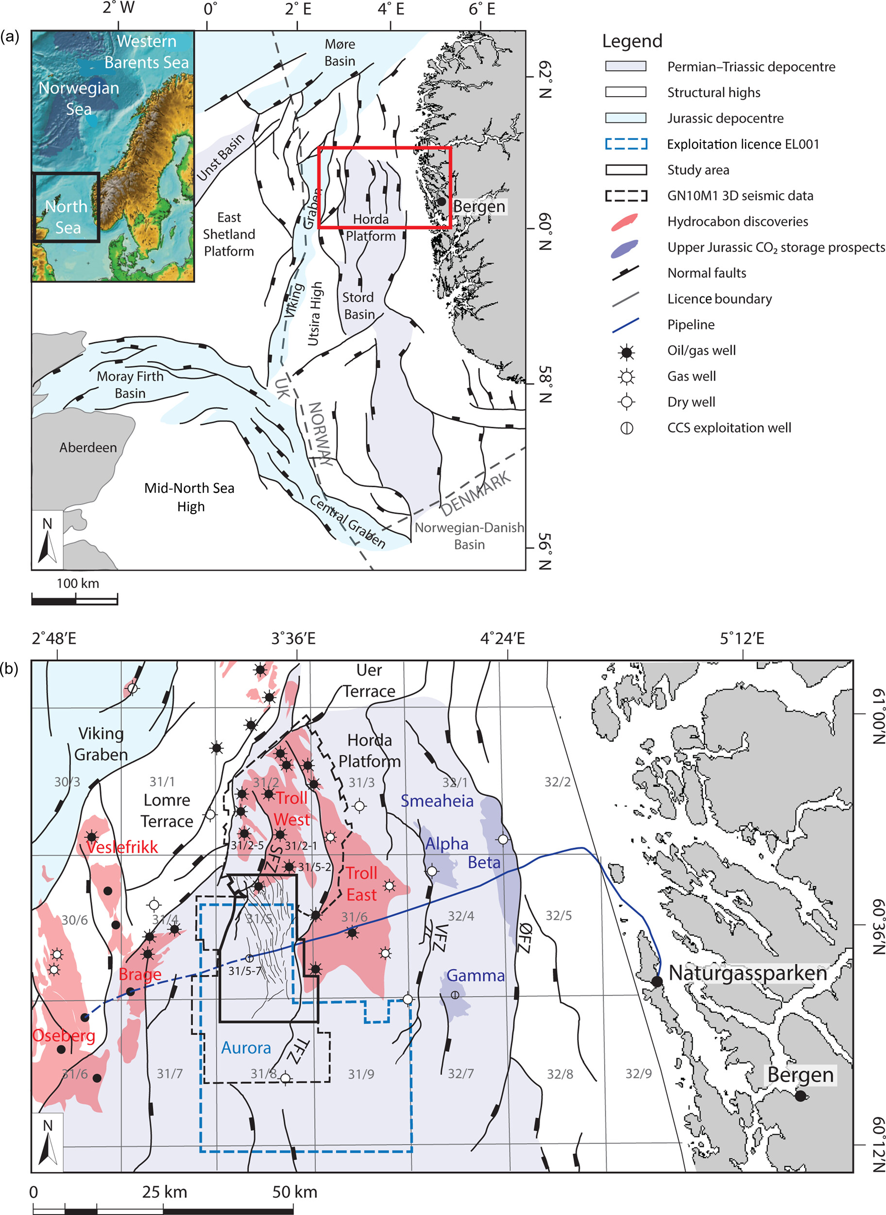
Fig. 111 Geological map of the North Sea highlighting the strike of normal faults around oil and gas fields, and formations targeted for carbon geological storage. Figure credit

Strike and dip of sedimentary strata can be reported in geological maps as shown in Fig. 112.

Fig. 112 Strike and dip in geological maps.

5.3 Frictional strength of faults and fault types

5.3.1 Fault strength

At the large scale, the Earth’s crust is constituted by “already broken” rock layers. These discontinuities are comprised mostly of faults. The cementation or cohesive strength of faults is negligible because the rock is already broken at those interfaces. Hence, a large block of rock does not have any cohesive strength or “unconfined compression strength”. As a result, its shear strength depends only on frictional strength according to the Coulomb frictional criterion (Fig. 113). You may think of “El Capitán” rock cliff (image here) as an example of a rock mass, strong and continuous, but that is an exception, not the rule. Furthermore, the size of “El Capitán” (\(\sim\) 900 m \(\sim\) 3000 ft) is smaller than the size of sedimentary basins (\(\sim\) 100 km and bigger).

Because of the lack of cohesive strength of the Earth’s crust at the large scale, its shear strength just depends on frictional strength through the friction coefficient \(\mu\) (or equivalent friction parameter \(q\)). The coefficient \(\mu_i\) is the internal frictional angle of rock before rupture, while \(\mu\) is the friction coefficient after initial rupture. Hence, the shear strength of large blocks in the Earth’s crust is simply

\[ \tau = \mu \: \sigma_n\]

which can be rewritten in terms of principal stresses as

\[ \sigma_1 = q \: \sigma_3\]

where

\[ q = \left( \sqrt{\mu^2 +1} + \mu \right) ^2 = \frac{1+\sin \: \varphi}{1-\sin \: \varphi}\]

For typical friction coefficients the coefficient \(q\) varies from 3 to 7. This means that the maximum ratio between maximum principal effective stress and minimum principal effective stress is \(\sigma_1/\sigma_3 \sim \) 3 to 7 (See Table \ref{table:FrictionAnisotropy}). This ratio is usually called “(effective) stress anisotropy”.

Fig. 113 Limits on effective principal stresses.

\caption{Relationship between friction coefficients, maximum stress anisotropy, and expected failure angle.}

\(\mu\)	\(q\)	\(\phi\)	\(\pi/4 + \phi/2\)
0.6	3.1	\(\sim 30^\circ\)	\(\sim 60^\circ\)
1.0	5.8	\(45^\circ\)	\(67.5^\circ\)
1.2	7.6	\(50^\circ\)	\(70^\circ\)

The maximum allowable stress anisotropy in a geological formation depends on its shear strength. Faults form or reactivate when this stress anisotropy, and therefore shear strength, is surpassed.

1. \(\sigma_1 / \sigma_3 > q\) implies fault slip.

2. \(\sigma_1 / \sigma_3 < q\) implies no fault slip.

These relationships can also be worked out in terms of total stresses but it is easier and more meaningful to keep them in terms of effective stresses (just do not forget about pore pressure).

5.3.2 Normal faults

A normal fault is caused by in-situ stress conditions in which

\[\begin{split} \left\lbrace \begin{array}{l} S_1 = S_v \\ S_2 = S_{Hmax} \\ S_3 = S_{hmin} \\ \end{array} \right.\end{split}\]

where \(S_1 > S_2 > S_3\). These stress conditions are typical of tectonically passive and laterally extensional environments. For example, the Permian Basin in Texas is mostly under normal faulting stress regime. The fault plane is a shear rupture plane. Its orientation is (\(\pi/4 + \varphi/2\)) in vertical direction from the horizontal plane (the plane perpendicular to \(S_v\)) to the plane of \(S_{hmin}\). The blocks move along the direction of \(S_v\) and do work against \(S_{hmin}\). At any point in the fault, the block above the fault is called the “hanging-wall” and the block below is the “footwall” (Fig. 114).

Fig. 114 Single normal fault.

Normal faults usually occur in pairs. Notice that the shear failure angle includes two possible solutions (for \(S_1 \neq S_2 \neq S_3\)). These are called conjugate solutions. The block that moves down in between two normal conjugate faults is termed “graben”, while the ones that move up relative to the footwall are called “horst” (Fig. 115). These geological structures occur frequently in hydrocarbon systems with structural fault traps.

Fig. 115 Conjugate normal faults forming graben and horst structures.

5.3.3 Thrust and reverse faults

A thrust fault is caused by in-situ stress conditions in which

\[\begin{split} \left\lbrace \begin{array}{l} S_1 = S_{Hmax} \\ S_2 = S_{hmin} \\ S_3 = S_v \\ \end{array} \right.\end{split}\]

These stress conditions are typical of locations with high compressive tectonic strains. For example, sedimentary basins close to the Andes and Himalayas foothills are under reverse faulting regime. The fault plane is a shear rupture plane. Its orientation is \((\pi/4 + \varphi/2)\) in vertical direction from a vertical plane perpendicular to \(S_{Hmax}\) to the plane of \(S_{v}\) (Fig. 116). The blocks move along the direction of \(S_{Hmax}\) and do work against gravity \(S_v\) (surface uplift). As with normal faulting, the block above the fault is called the “hanging-wall” and the block below the “footwall”.

Fig. 116 Thrust fault example

A fault that may have been caused by paleo-stresses corresponding to a normal stress regime, but now moves according to in-situ stress conditions of a thrust fault stress environment is termed a reverse fault (Fig. 117).

Fig. 117 Reverse fault example.

5.3.4 Strike-slip faults

A strike-slip fault is caused by in-situ stress conditions in which

\[\begin{split} \left\lbrace \begin{array}{l} S_1 = S_{Hmax} \\ S_2 = S_v \\ S_3 = S_{hmin} \\ \end{array} \right.\end{split}\]

These stress conditions are typical of high compressive tectonic strains mostly in one direction. Some sedimentary basins around the Rocky Mountains and near California are under strike slip regime. The fault plane is a shear rupture plane and it is vertical. Its orientation is \((\pi/4 + \varphi/2)\) in horizontal direction from a vertical plane perpendicular to \(S_{Hmax}\) towards a plane perpendicular to \(S_{hmin}\). The schematic in Fig. 118 shows an oblique fault, not a pure strike-slip fault. The fault is called strike-slip, because it slips in horizontal direction, in the direction of the fault strike. Notice that oblique faults move with a combination of vertical and horizontal displacements.

Fig. 118 Strike-slip fault example.

5.3.5 Stress and faulting regimes

The type of fault that occurs for each stress combination gives rise to the name of the stress faulting regime (Table \ref{table:Andersonian}). Notice that stresses may change in magnitude and direction with time at a given location (see stress map in Fig. 119 - other maps available at \url{http://www.world-stress-map.org/}). Furthermore, the same location may evolve through different stress regimes over geological periods of time. The stress regime can also change with depth at the same location. Changes of stress regime with depth are critical for defining the geometry of fluid-driven fractures.

\caption{The Andersonian faulting classification system.} \label{table:Andersonian}

Faulting regime	Maximum principal stress \(S_1\)	Intermediate principal stress \(S_2\)	Minimum principal stress \(S_3\)
Normal (NF)	\(S_v\)	\(S_{Hmax}\)	\(S_{hmin}\)
Strike-slip (SS)	\(S_{Hmax}\)	\(S_v\)	\(S_{hmin}\)
Reverse (RF)	\(S_{Hmax}\)	\(S_{hmin}\)	\(S_v\)

Fig. 119 World stress map. The figure above shows directions of maximum horizontal stresses based on various types of field measurements. The orientation of maximum horizontal stress varies with location and is strongly influenced by plate movement and imparted tectonic strains.

5.3.6 Ideal orientation of faults

The ideal orientation of a hydraulic fracture is a plane perpendicular to the minimum principal stress \(S_3\) direction. Similarly, we can also tell what would be the orientation of ideal conjugate pairs of shear fractures (faults) for a given state of stress. The dip and strike will depend on \(S_1\), \(S_3\), and the friction angle \(\varphi\) (Fig. 121). Such ideal conjugate pair of shear fractures would be located:

1. in planes that are in between the planes perpendicular to \(S_1\) and \(S_3\),

2. in planes that are co-linear with \(S_2\),

3. in planes that are at \(\pi/4 + \varphi/2\) from the plane perpendicular to \(S_1\) towards the plane perpendicular to \(S_3\).

The general solution is shown in Fig. 120.

Fig. 120 Ideal orientation of a pair of conjugate shear fractures (faults) as a function of the orientation of principal stresses and the friction angle.

Notice that all these angles vary according to the stress regime. Faults formed in NF stress regime tend to be steep. Faults formed in RF stress regime are not too steep. Faults formed in SS stress regime are vertical.

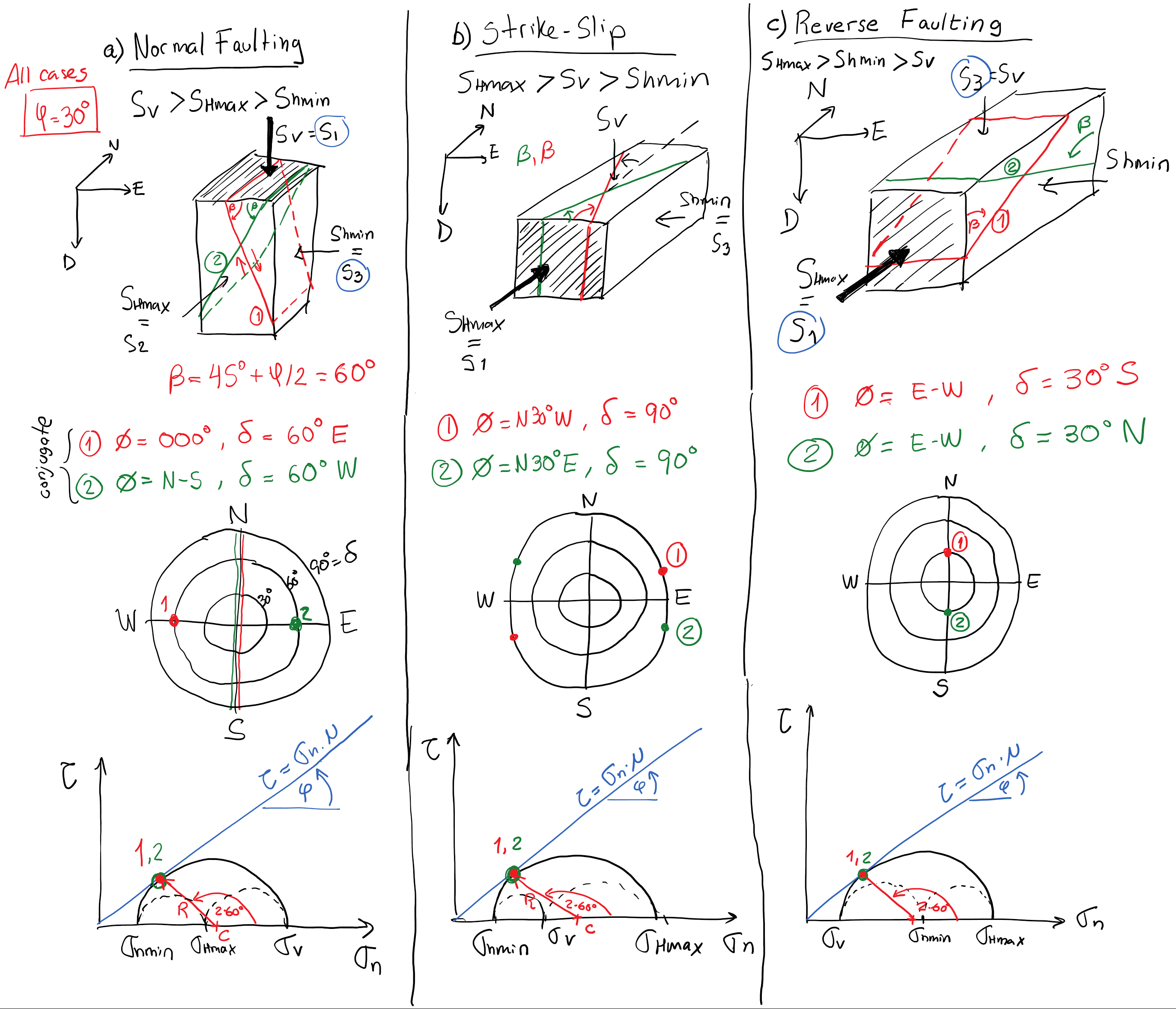
Fig. 121 Summary of ideal pairs of shear fractures in (left) normal fault stress regime, (center) strike-slip stress regime, and (right) thrust (reverse) faulting stress regime. From top to bottom the figure shows: block diagrams with stresses, block diagram with shear fractures, stereonets, and 3D Mohr circles.

Example 5.1

Find the ideal orientation of a hydraulic fracture and faults (shear fractures) at a location subjected to the following state of stress and conditions:

• Stress regime: Normal faulting

• \(S_v\) is a principal stress

• Azimuth of \(S_{hmin}\) is N60\(^{\circ}\)W

• Friction angle \(\varphi\) = 30\(^{\circ}\).

SOLUTION

First, recognize the planes of \(S_1\) and \(S_3\) and their orientations with respect to the geographical coordinate system. The plane of \(S_1\) in this case is a horizontal plane (\(S_v\) plane, a principal stress) and the plane of \(S_3\) is a vertical plane perpendicular to \(S_{hmin}\).

Fig. 122 Example 5.1 solution.

A hydraulic fracture would be perpendicular to \(S_3\), in this case \(S_{hmin}\). Hence, the strike is \(\phi_{HF} = 030^{\circ}\) and the dip is \(\delta_{HF} = 90^{\circ}\) because \(S_3\) is horizontal.

The dip of faults depends on the friction angle. In this case, the failure angle is: \(\beta = 45^{\circ} + \varphi / 2 = 45^{\circ} + 30^{\circ} / 2 = 60^{\circ} \). The fault planes are at \(\beta\) going from the plane of \(S_1\) to the plane of \(S_3\). Thus, the strike of the two possible faults is \(\phi_{F1} = \phi_{F2} = 030^{\circ}\) and the dips are \(\delta_{F1} = 60^{\circ}\)SE and \(\delta_{F1} = 60^{\circ}\)NW. \(\: \: \blacksquare\)

Example 5.2

Find the ideal orientation of a hydraulic fracture and faults (shear fractures) at a location subjected to the following state of stress and conditions:

• Stress regime: Strike-slip faulting

• \(S_v\) is a principal stress

• Azimuth of \(S_{Hmax}\) is 010\(^{\circ}\)

• Friction angle \(\varphi\) = 40\(^{\circ}\).

SOLUTION

First, recognize the planes of \(S_1\) and \(S_3\) and their orientations with respect to the geographical coordinate system. The plane of \(S_1\) in this case is a vertical plane (\(S_{Hmax}\) plane) and the plane of \(S_3\) is another vertical plane perpendicular to \(S_{hmin}\).

Fig. 123 Example 5.2 solution.

A hydraulic fracture would be perpendicular to \(S_3\), in this case \(S_{hmin}\). Hence, the strike is \(\phi_{HF} = 010^{\circ}\) and the dip is \(\delta_{HF} = 90^{\circ}\) because \(S_3\) is horizontal.

The dip of faults depends on the friction angle. In this case, the failure angle is: \( \beta = 45^{\circ} + \varphi / 2 = 45^{\circ} + 40^{\circ} / 2 = 65^{\circ} \). The fault planes are at \(\beta\) going from the plane of \(S_1\) to the plane of \(S_3\). Thus, the strikes of the two possible faults are \(\phi_{F1} = 345^{\circ}\) and \(\phi_{F2} = 035^{\circ}\), the dip is \(\delta_{F1} = \delta_{F2} = 90^{\circ}\). \(\: \: \blacksquare\)

5.4 Determination of normal and shear stresses on the fault plane

In this section we will review two methods to calculate normal and shear stresses on fractures and faults. The first part reviews the Mohr circle method in order to have a conceptual understanding of stress projection on faults and maximum ratio between shear stress and effective normal stress. The second part discusses the tensor method, which requires the definition of three coordinate systems and matrix multiplication. The tensor method can be easily implemented in a computer script but is laborious to work out manually.

5.4.1 Mohr’s circle method

The 3D Mohr circle is a graphical representation of the stress tensor and all its projections (or possibles values of normal effective stress \(\sigma_n\) and shear stress \(\tau\)) on a given plane. Consider a horizontal plane in Fig. 124, the normal stress is the vertical stress \(S_v\) and there is no shear stress. Consider a vertical plane with strike East-West in Fig. 124, you get the minimum principal stress \(S_{hmin}\). Consider a vertical plane with strike North-South in Fig. 124, you get the maximum principal stress \(S_{Hmax}\).

Likewise, non-trivial solutions of stress projection at an arbitrary plane angle include all the points delimited by the three Mohr circles. Let’s consider solutions along each circle in Fig. 124.

1. The blue circle (center C\(_1\)) represents the possible state of stresses that result as a combination of \(\sigma_v\) and \(\sigma_{hmin}\). The shear stress \(\tau\) and normal effective stress \(\sigma_n\) of any plane in between the planes of \(\sigma_v\) and \(\sigma_{hmin}\) and colinear with \(\sigma_{Hmax}\) can be found through the angle \(\beta_1\) measured from \(\sigma_v\).

2. The green circle (center C\(_2\)) represents the possible state of stresses that result as a combination of \(\sigma_{v}\) and \(\sigma_{Hmax}\). The shear stress \(\tau\) and normal effective stress \(\sigma_n\) of any plane in between the planes of \(\sigma_{v}\) and \(\sigma_{Hmax}\) and colinear with \(\sigma_{hmin}\) can be found through the angle \(\beta_2\) measured from \(\sigma_v\)

3. The red circle (center C\(_3\)) represents the possible state of stresses that result as a combination of \(\sigma_{Hmax}\) and \(\sigma_{hmin}\). The shear stress \(\tau\) and normal effective stress \(\sigma_n\) of any plane in between the planes of \(\sigma_{Hmax}\) and \(\sigma_{hmin}\) and colinear with \(\sigma_{v}\) can be found through the angle \(\beta_3\) measured from \(\sigma_{Hmax}\)

Fig. 124 The 3D Mohr circle

For this example (normal faulting, \(S_{Hmax}\) azimuth E-W), an ideal fault would occur with a strike E-W and dip 60\(^{\circ}\) (assuming \(\varphi = 30^{\circ}\)). This is the orientation of a plane with maximum \(\tau/\sigma_n\).

Example 5.3

Find the shear and normal effective stresses on a fault plane within the following state of stress and conditions:

• Fault: strike azimuth = 000\(^{\circ}\), dip = 60\(^{\circ}\).

• State of stress: \(S_v =\) 23 MPa (principal), \(S_{Hmax} =\) 20 MPa, \(S_{hmin} =\) 13.8 MPa (azimuth: 090\(^{\circ}\)), and \(P_p =\) 10 MPa.

SOLUTION

Fig. 125 Problem Ex. 5.3

The effective stresses are: \(\sigma_v =\) 13 MPa, \(\sigma_{Hmax} =\) 10 MPa, \(\sigma_{hmin} =\) 3.8 MPa. Based on the Mohr circle of \(\sigma_v\) with \(\sigma_{hmin}\) and trigonometry:

\( \sigma_n = \left( \frac{13 \text{ MPa} + 3.8 \text{ MPa}}{2} \right) + \left( \frac{13 \text{ MPa} - 3.8 \text{ MPa}}{2} \right) \cos(2 \cdot 60^{\circ}) = 6.1 \text{ MPa} \)

\( \tau = \left( \frac{13 \text{ MPa} - 3.8 \text{ MPa}}{2} \right) \sin(2 \cdot 60^{\circ}) = 4.0 \text{ MPa} \: \: \blacksquare \)

Example 5.4

Find the shear and normal effective stresses on a fault plane within the following state of stress and conditions:

• Fault: strike azimuth = N60\(^{\circ}\)E, dip: 90\(^{\circ}\).

• State of stress: \(S_v =\) 30 MPa (principal), \(S_{Hmax} =\) 45 MPa, \(S_{hmin} =\) 25 MPa (azimuth: N30\(^{\circ}\)E), and \(P_p =\) 15 MPa.

SOLUTION

Fig. 126 Problem Ex. 5.4

The effective stresses are: \(\sigma_v =\) 15 MPa, \(\sigma_{Hmax} =\) 30 MPa, \(\sigma_{hmin} =\) 10 MPa. Based on the Mohr circle of \(\sigma_{Hmax}\) with \(\sigma_{hmin}\) and trigonometry:

\( \sigma_n = \left( \frac{30 \text{ MPa} + 10 \text{ MPa}}{2} \right) + \left( \frac{30 \text{ MPa} - 10 \text{ MPa}}{2} \right) \cos(2 \cdot 30^{\circ}) = 25 \text{ MPa} \)

\( \tau = \left( \frac{30 \text{ MPa} - 10 \text{ MPa}}{2} \right) \sin(2 \cdot 30^{\circ}) = 8.7 \text{ MPa} \: \: \blacksquare \)

5.4.2 Tensor method

This subsection describes the procedure to calculate stresses \((\sigma_n, \tau)\) on an arbitrary plane given its orientation respect to the geographical coordinate system \((strike,dip)\) and the in-situ stress tensor of principal stresses \(\underset{=}{S}{}_P\) (given its principal values and principal directions).

The first step consists on defining the principal stress coordinate system and the geographical coordinate system (both right-handed coordinate systems).

• The principal stress coordinate system has the three principal directions as bases of the system in the order of most compressive to least compressive: \(\underline{e}_1\) for \(S_1\), \(\underline{e}_2\) for \(S_2\), and \(\underline{e}_3\) for \(S_3\) (Fig. 127). The stress tensor is termed \(\underset{=}{S}{}_P\) in this coordinate system.

• The geographical coordinate system has bases \(\underline{e}_1\) pointing in North direction, \(\underline{e}_2\) pointing in East direction, and \(\underline{e}_3\) pointing down in direction of increasing depth (Fig. 127). We will refer this basis as the “NED” basis. The stress tensor is termed \(\underset{=}{S}{}_G\) in this coordinate system.

Fig. 127 The stress tensor in principal directions and geographical coordinate systems.

The \textit{second step} involves constructing a change of basis matrix \(R_{PG}\) from the Principal Stress to the Geographical Coordinate system. This matrix depends on the projections of the elements of the new base on the old base according to the cosines of the director angles \(\alpha\), \(\beta \), and \(\gamma\) (Fig. 128). Table \ref{table:RPGsummary} summarizes the meaning of \(\alpha\), \(\beta \), and \(\gamma\) for cases in which vertical stress is a principal stress.

Fig. 128 Transformation matrix from the principal directions to geographical coordinate system and corresponding angles.

(43)\[\begin{split} R_{PG} = \left[ \begin{array}{ccc} \cos \alpha \cos \beta & \sin \alpha \cos \beta & -\sin \beta \\ \cos \alpha \sin \beta \sin \gamma - \sin \alpha \cos \gamma & \sin \alpha \sin \beta \sin \gamma + \cos \alpha \cos \gamma & \cos \beta \sin \gamma \\ \cos \alpha \sin \beta \cos \gamma + \sin \alpha \sin \gamma & \sin \alpha \sin \beta \cos \gamma - \cos \alpha \sin \gamma & \cos \beta \cos \gamma \end{array} \right]\end{split}\]

\caption{Summary of possible values of \(\alpha\), \(\beta\), and \(\gamma\) for vertical stress being a principal stress. Notes: (1) these angles indicate solely the orientation of principal stresses with respect to the geographical coordinate system, (2) this \(\beta\) has nothing to do with the angle used in the Mohr’s circle method to solve for stresses on a fault.} \label{table:RPGsummary}

	Normal faulting	Strike slip	Reverse faulting
\(\alpha\)	Azimuth of \(S_{hmin}\)	Azimuth of \(S_{Hmax}\)	Azimuth of \(S_{Hmax}\)
\(\beta\)	\(90^\circ\)	\(0^\circ\)	\(0^\circ\)
\(\gamma\)	\(0^\circ\)	\(90^\circ\)	\(0^\circ\)

Check out this link for an animation of \(\alpha\), \(\beta \), and \(\gamma\) in arbitrary directions.

With the matrix \(R_{PG}\), we can calculate the stress tensor \(\underset{=}{S}{}_P\) as a function of \(\underset{=}{S}{}_G\),

\[ \underset{=}{S}{}_P = R_{PG} \underset{=}{S}{}_G R_{PG}^T\]

and therefore:

(44)\[ \underset{=}{S}{}_G = R_{PG}^T \underset{=}{S}{}_P R_{PG}\]

where the superscript \(T\) stands for “transpose”.

Example 5.5

Calculate \(\underset{=}{S}{}_G\) in a normal faulting stress regime case (\(S_1 = 30\) MPa, \(S_2 = 25\) MPa, \(S_3 = 20\) MPa) with azimuth of \(S_{hmin}\) N-S. \(S_v\) is a principal stress.

SOLUTION

The principal stress tensor is

\( \underset{=}{S}{}_P = \left[ \begin{array}{ccc} 30 & 0 & 0 \\ 0 & 25 & 0 \\ 0 & 0 & 20 \end{array} \right] \)

Using Table \ref{table:RPGsummary} and considering that \(S_1 = S_v\), the angles of the principal stress coordinate result \(\alpha = 0^{\circ}\), \(\beta = 90^{\circ}\), and \(\gamma = 0^{\circ}\). The change of coordinate system matrix results

\( R_{PG} = \left[ \begin{array}{ccc} 0 & 0 & -1 \\ 0 & 1 & 0 \\ 1 & 0 & 0 \end{array} \right] \)

Finally, using equation \ref{eq:SGcalc}

\( \underset{=}{S}{}_G = \left[ \begin{array}{ccc} 0 & 0 & -1 \\ 0 & 1 & 0 \\ 1 & 0 & 0 \end{array} \right]^T \: \left[ \begin{array}{ccc} 30 & 0 & 0 \\ 0 & 25 & 0 \\ 0 & 0 & 20 \end{array} \right] \: \left[ \begin{array}{ccc} 0 & 0 & -1 \\ 0 & 1 & 0 \\ 1 & 0 & 0 \end{array} \right] = \left[ \begin{array}{ccc} 20 & 0 & 0 \\ 0 & 25 & 0 \\ 0 & 0 & 30 \end{array} \right] \: \: \blacksquare \)

Example 5.6

Calculate \(\underset{=}{S}{}_G\) in a strike-slip faulting stress regime case (\(S_1 = 30\) MPa, \(S_2 = 25\) MPa, \(S_3 = 20\) MPa) with azimuth of \(S_{Hmax}\) N-S. \(S_v\) is a principal stress.

SOLUTION

The principal stress tensor is

\( \underset{=}{S}{}_P = \left[ \begin{array}{ccc} 30 & 0 & 0 \\ 0 & 25 & 0 \\ 0 & 0 & 20 \end{array} \right] \)

Using Table \ref{table:RPGsummary} and considering that \(S_1 = S_{Hmax}\) and \(S_2 = S_v\), the angles of the principal stress coordinate result \(\alpha = 0^{\circ}\), \(\beta = 0^{\circ}\), and \(\gamma = 90^{\circ}\). The change of coordinate system matrix results

\( R_{PG} = \left[ \begin{array}{ccc} 1 & 0 & 0 \\ 0 & 0 & 1 \\ 0 & -1 & 0 \end{array} \right] \)

Finally, using equation \ref{eq:SGcalc}

\( \underset{=}{S}{}_G = \left[ \begin{array}{ccc} 1 & 0 & 0 \\ 0 & 0 & 1 \\ 0 & -1 & 0 \end{array} \right]^T \: \left[ \begin{array}{ccc} 30 & 0 & 0 \\ 0 & 25 & 0 \\ 0 & 0 & 20 \end{array} \right] \: \left[ \begin{array}{ccc} 1 & 0 & 0 \\ 0 & 0 & 1 \\ 0 & -1 & 0 \end{array} \right] = \left[ \begin{array}{ccc} 30 & 0 & 0 \\ 0 & 20 & 0 \\ 0 & 0 & 25 \end{array} \right] \: \: \blacksquare \)

Example 5.7

Calculate \(\underset{=}{S}{}_G\) in a reverse faulting stress regime case (\(S_1 = 30\) MPa, \(S_2 = 25\) MPa, \(S_3 = 20\) MPa) with azimuth of \(S_{Hmax}\) E-W. \(S_v\) is a principal stress.

SOLUTION

The principal stress tensor is

\( \underset{=}{S}{}_P = \left[ \begin{array}{ccc} 30 & 0 & 0 \\ 0 & 25 & 0 \\ 0 & 0 & 20 \end{array} \right] \)

Using Table \ref{table:RPGsummary} and considering that \(S_1 = S_{Hmax}\) and \(S_2 = S_{hmin}\), the angles of the principal stress coordinate result \(\alpha = 90^{\circ}\), \(\beta = 0^{\circ}\), and \(\gamma = 0^{\circ}\). The change of coordinate system matrix results

\( R_{PG} = \left[ \begin{array}{ccc} 0 & 1 & 0 \\ -1 & 0 & 0 \\ 0 & 0 & 1 \end{array} \right] \)

Finally, using equation \ref{eq:SGcalc}

\( \underset{=}{S}{}_G = \left[ \begin{array}{ccc} 0 & 1 & 0 \\ -1 & 0 & 0 \\ 0 & 0 & 1 \end{array} \right]^T \: \left[ \begin{array}{ccc} 30 & 0 & 0 \\ 0 & 25 & 0 \\ 0 & 0 & 20 \end{array} \right] \: \left[ \begin{array}{ccc} 0 & 1 & 0 \\ -1 & 0 & 0 \\ 0 & 0 & 1 \end{array} \right] = \left[ \begin{array}{ccc} 25 & 0 & 0 \\ 0 & 30 & 0 \\ 0 & 0 & 20 \end{array} \right] \: \: \blacksquare \)

Example 5.8

Calculate \(\underset{=}{S}{}_G\) in a strike-slip faulting stress regime case (\(S_1 = 60\) MPa, \(S_2 = 40\) MPa, \(S_3 = 35\) MPa) with azimuth of \(S_{Hmax}\) being 135\(^{\circ}\). \(S_v\) is a principal stress.

SOLUTION

The principal stress tensor is

\( \underset{=}{S}{}_P = \left[ \begin{array}{ccc} 60 & 0 & 0 \\ 0 & 40 & 0 \\ 0 & 0 & 35 \end{array} \right] \)

Using Table \ref{table:RPGsummary} and considering that \(S_1 = S_{Hmax}\) and \(S_2 = S_v\), the angles of the principal stress coordinate result \(\alpha = 135^{\circ}\), \(\beta = 0^{\circ}\), and \(\gamma = 90^{\circ}\). The change of coordinate system matrix results

\( R_{PG} = \left[ \begin{array}{ccc} -0.707 & 0.707 & 0 \\ 0 & 0 & 1 \\ 0.707 & 0.707 & 0 \end{array} \right] \)

Finally, using equation \ref{eq:SGcalc}

\( \underset{=}{S}{}_G = \left[ \begin{array}{ccc} -0.707 & 0.707 & 0 \\ 0 & 0 & 1 \\ 0.707 & 0.707 & 0 \end{array} \right]^T \: \left[ \begin{array}{ccc} 60 & 0 & 0 \\ 0 & 40 & 0 \\ 0 & 0 & 35 \end{array} \right] \: \left[ \begin{array}{ccc} -0.707 & 0.707 & 0 \\ 0 & 0 & 1 \\ 0.707 & 0.707 & 0 \end{array} \right] = \left[ \begin{array}{ccc} 47.5 & -12.5 & 0 \\ -12.5 & 47.5 & 0 \\ 0 & 0 & 40 \end{array} \right] \: \: \blacksquare \)

The third step consists in defining the fault plane coordinate system. The coordinate system basis is comprised of \(n_d\) (dip), \(n_s\) (strike), and \(n_n\) (normal) vectors: d-s-n right-handed basis. The three vectors depend solely in two variables: \(strike\) and \(dip\) of the fault.

Fig. 129 Fault coordinate system as a function of strike and dip.

The fourth step (and last) consists in projecting the stress tensor based on the geographical coordinate system onto the fault base vectors. The stress vector acting on the plane of the fault is \(\underline{t}\) (note that \(\underline{t}\) is not necessarily aligned with \(\underline{n}_d\), \(\underline{n}_s\) or \(\underline{n}_n\)) and is calculated according to:

\[ \underline{t} = \underset{=}{S}{}_G \underline{n}_n\]

The total normal stress on the plane of the fault is \(S_n\) (aligned with \(\underline{n}_n\)):

\[ S_n = \underline{t} \cdot \underline{n}_n\]

The effective normal stress on the fault plane is \(\sigma_n = S_n - P_p \). The shear stresses on the plane of the fault is aligned with \(\underline{n}_d\) and \(\underline{n}_s\) are:

\[\begin{split} \left\lbrace \begin{array}{l} \tau_d = \underline{t} \cdot \underline{n}_d \\ \tau_s = \underline{t} \cdot \underline{n}_s \end{array} \right.\end{split}\]

The dot product is used in all these vector to vector multiplications. The geometrical meaning is the projection of one vector onto the other.

The effective normal stress \(\sigma_n\) and absolute shear \(\tau = \sqrt{\tau_d^2 + \tau_s^2}\) can also be calculated with the following equations:

\[ \sigma_n = \underline{t} \cdot \underline{n}_n - P_p\]

\[ \tau^2 = ||\underline{t}||^2 - ||\underline{t} \cdot \underline{n}_n||^2\]

The \(rake\) is the angle of the shear stress \(\underline{\tau}_d + \underline{\tau}_s\) with respect to \(\underline{n}_s\) (horizontal line) and quantifies the direction of expected fault movement in the fault plane.

\[ rake = \arctan \left( \frac{\tau_d}{\tau_s} \right)\]

Example 5.9

Calculate \(t\), \(S_n\), \(\tau_d\), \(\tau_s\), and \(rake\) for a fault with strike 000\(^{\circ}\) and dip 60\(^{\circ}\)E in a place with normal faulting stress regime (\(S_v = 23\) MPa, \(S_{Hmax} = 15\) MPa, \(S_{hmin} = 13.8\) MPa) with azimuth of \(S_{hmin}\) equal to 90\(^{\circ}\). \(S_v\) is a principal stress.

SOLUTION

The tensor of principal stresses is

\( \underset{=}{S}{}_P = \left[ \begin{array}{ccc} 23 & 0 & 0 \\ 0 & 15 & 0 \\ 0 & 0 & 13.8 \end{array} \right] \)

Using Table \ref{table:RPGsummary} and considering that \(S_1 = S_v\) and the azimuth of \(S_{hmin}\) is 90\(^{\circ}\), the angles of the principal stress coordinate result \(\alpha = 90^{\circ}\), \(\beta = 90^{\circ}\), and \(\gamma = 0^{\circ}\). The change of coordinate system matrix results

\( R_{PG} = \left[ \begin{array}{ccc} 0 & 0 & -1 \\ -1 & 0 & 0 \\ 0 & 1 & 0 \end{array} \right] \)

and the total stress in the geographical coordinate system results

\( \underset{=}{S}{}_G = \left[ \begin{array}{ccc} 15 & 0 & 0 \\ 0 & 13.8 & 0 \\ 0 & 0 & 23 \end{array} \right] \)

Given the orientation of the fault, the vector normal to the fault is

\( \underline{n}{}_n = \left[ \begin{array}{c} 0 \\ 0.867 \\ -0.5 \end{array} \right] \)

Finally, the stresses on the fault are

\(\underline{t}= [0,11.95,-11.50]\) MPa.\newline \(S_n = 16.1\) MPa \newline \(\tau_d = -3.98\) MPa \newline \(\tau_s = 0\) MPa \newline \(rake\) = 90\(^{\circ} \: \: \blacksquare \) \newline

Example 5.10

Calculate \(t\), \(S_n\), \(\tau_d\), \(\tau_s\), and \(rake\) for a fault with strike 060\(^{\circ}\) and dip 90\(^{\circ}\) in a place with strike-slip stress regime (\(S_v = 30\) MPa, \(S_{Hmax} = 45\) MPa, \(S_{hmin} = 25\) MPa) with azimuth of \(S_{Hmax}\) equal to 120\(^{\circ}\). \(S_v\) is a principal stress.

SOLUTION

The tensor of principal stresses is

\( \underset{=}{S}{}_P = \left[ \begin{array}{ccc} 45 & 0 & 0 \\ 0 & 30 & 0 \\ 0 & 0 & 25 \end{array} \right] \text{ MPa} \)

Using Table \ref{table:RPGsummary} and considering that \(S_1 = S_v\) and the azimuth of \(S_{Hmax}\) is 120\(^{\circ}\), the angles of the principal stress coordinate result \(\alpha = 120^{\circ}\), \(\beta = 0^{\circ}\), and \(\gamma = 90^{\circ}\). The change of coordinate system matrix results

\( R_{PG} = \left[ \begin{array}{ccc} -0.5 & 0.866 & 0 \\ 0 & 0 & 1 \\ 0.866 & 0.5 & 0 \end{array} \right] \)

and the total stress in the geographical coordinate system results

\( \underset{=}{S}{}_G = \left[ \begin{array}{ccc} 30 & -8.66 & 0 \\ -8.66 & 40 & 0 \\ 0 & 0 & 30 \end{array} \right] \text{ MPa} \)

Given the orientation of the fault, the vector normal to the fault is

\( \underline{n}{}_n = \left[ \begin{array}{c} -0.866 \\ 0.5 \\ 0 \end{array} \right] \)

Finally, the stresses on the fault are

\(\underline{t}= [-30.31,27.5,0]\) MPa.\newline \(S_n = 40\) MPa \newline \(\tau_d = 0\) MPa \newline \(\tau_s = 8.66\) MPa \newline \(rake\) = 0\(^{\circ} \: \: \blacksquare \) \newline

Example 5.11

Calculate \(t\), \(S_n\), \(\tau_d\), \(\tau_s\), and \(rake\) for conjugate faults with strike 045\(^{\circ}\) and 225\(^{\circ}\) both with dip 60\(^{\circ}\) in a place with normal faulting stress regime (\(S_v = 5000\) psi, \(S_{Hmax} = 4000\) psi, \(S_{hmin} = 3000\) psi) with azimuth of \(S_{hmin}\) equal to 90\(^{\circ}\). \(S_v\) is a principal stress.

SOLUTION

The tensor of principal stresses is

\( \underset{=}{S}{}_P = \left[ \begin{array}{ccc} 5000 & 0 & 0 \\ 0 & 4000 & 0 \\ 0 & 0 & 3000 \end{array} \right] \text{ psi} \)

Using Table \ref{table:RPGsummary} and considering that \(S_1 = S_v\) and the azimuth of \(S_{hmin}\) is 90\(^{\circ}\), the angles of the principal stress coordinate result \(\alpha = 90^{\circ}\), \(\beta = 90^{\circ}\), and \(\gamma = 0^{\circ}\). The change of coordinate system matrix results

\( R_{PG} = \left[ \begin{array}{ccc} 0 & 0 & -1 \\ -1 & 0 & 0 \\ 0 & 1 & 0 \end{array} \right] \)

and the total stress tensor in the geographical coordinate system results

\( \underset{=}{S}{}_G = \left[ \begin{array}{ccc} 4000 & 0 & 0 \\ 0 & 3000 & 0 \\ 0 & 0 & 5000 \end{array} \right] \text{ psi} \)

Let us consider the first fault with strike of 045\(^{\circ}\) and dip of 60\(^{\circ}\), the vector normal to the faults is

\( \underline{n}{}_{n} = \left[ \begin{array}{c} -0.612 \\ 0.612 \\ -0.5 \end{array} \right] \)

The stresses on this fault are

\(\underline{t}= [-2450,1840,-2500]\) psi.\newline \(S_n = 3870\) psi \newline \(\tau_d = -649\) psi \newline \(\tau_s = -433\) psi \newline \(rake\) = 56.3\(^{\circ}\)\newline

Let us consider the fault with strike of 225\(^{\circ}\) and dip of 60\(^{\circ}\), the vector normal to the faults is

\( \underline{n}{}_{n} = \left[ \begin{array}{c} 0.612 \\ -0.612 \\ -0.5 \end{array} \right] \)

The stresses on this fault are

\(\underline{t}= [2450,-1840,-2500]\) psi.\newline \(S_n = 3870\) psi \newline \(\tau_d = -649\) psi \newline \(\tau_s = -433\) psi \newline \(rake\) = 56.3\(^{\circ} \: \: \blacksquare \) \newline

Example 5.12

Calculate \(t\), \(S_n\), \(\tau_d\), \(\tau_s\), \(rake\), and \(\tau / \sigma_n\) for a fault with strike 120\(^{\circ}\) and 70\(^{\circ}\) dip in a place with reverse faulting stress regime (\(S_v = 1000\) psi, \(S_{Hmax} = 2400\) psi, \(S_{hmin} = 1200\) psi) with azimuth of \(S_{Hmax}\) equal to 150\(^{\circ}\) and pore pressure \(P_p = 440\) psi. \(S_v\) is a principal stress.

SOLUTION

The tensor of principal stresses is

\( \underset{=}{S}{}_P = \left[ \begin{array}{ccc} 2400 & 0 & 0 \\ 0 & 1200 & 0 \\ 0 & 0 & 1000 \end{array} \right] \text{ psi} \)

and the pore pressure is \(P_p = 440\) psi.

Using Table \ref{table:RPGsummary} and considering that \(S_3 = S_v\) and the azimuth of \(S_{Hmax}\) is 150\(^{\circ}\), the angles of the principal stress coordinate result \(\alpha = 150^{\circ}\), \(\beta = 0^{\circ}\), and \(\gamma = 0^{\circ}\). The change of coordinate system matrix results

\( R_{PG} = \left[ \begin{array}{ccc} -0.866 & 0.5 & 0 \\ -0.5 & -0.866 & 0 \\ 0 & 0 & 1 \end{array} \right] \)

and the total stress in the geographical coordinate system results

\( \underset{=}{S}{}_G = \left[ \begin{array}{ccc} 2100 & -520 & 0 \\ -520 & 1500 & 0 \\ 0 & 0 & 1000 \end{array} \right] \text{ psi} \)

Given the orientation of the fault, the vector normal to the fault is

\( \underline{n}{}_n = \left[ \begin{array}{c} -0.814 \\ -0.470 \\ -0.342 \end{array} \right] \)

Finally, the stresses on the fault are

\(\underline{t}= [-1465,-281,-342]\) psi.\newline \(S_n = 1441\) psi, \(\sigma_n = 1001\) psi \newline \(\tau_d = 160\) psi, \(\tau_s = 488\) psi, \(\tau = 514\) psi \newline \(rake\) = 18.21\(^{\circ}\) \newline

The ratio of shear to normal effective stress is \(\tau / \sigma_n = 0.51 \: \: \blacksquare\)

Example: make 3D Mohr-Circle filled with color corresponding to \(\tau / \sigma_n\) value, stereo net, and fractures in 3D.

5.5 Applications

5.5.1 Critically stressed fractures and permeability

The previous section shows how to calculate the normal effective stress \(\sigma_n\) and shear stress \(\tau\) components on an arbitrary oriented plane given the in-situ state of stress. A critically-stressed fracture (or fault) has shear stress and normal effective stress components with a ratio \(\tau/\sigma_n\) which approaches the friction coefficient \(\mu \sim\) 0.6-1.0. The fracture is said to be ``critically stressed’’ because it is practically failing in shear. Such fractures -if they exhibit dilation during sliding- tend to be more hydraulically conductive than fractures with low \(\tau/\sigma_n\) ratio (on the right of the Mohr circle and far left close to \(\sigma_3\) - Fig. 132). Natural fractures can help fluid drainage. Traditionally, fracture permeability has been thought to be dependent on effective normal stress only \(k_{frac} = f(\sigma_n)\). The concept of critically stressed fractures adds one more level of dependency to fracture permeability such that it is also a function of shear stress \(k_{frac} = f(\sigma_n,\tau)\).

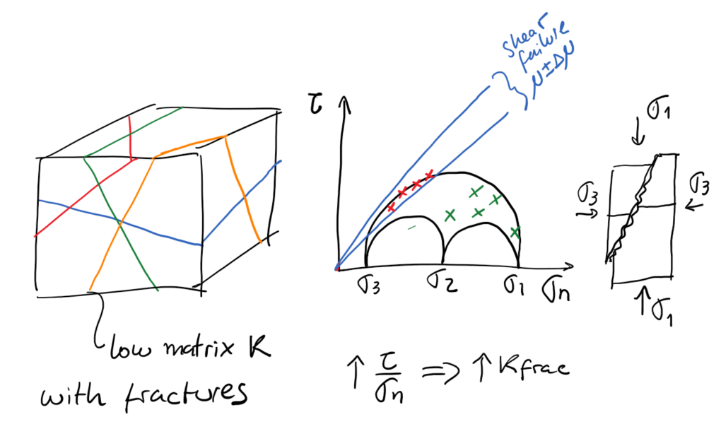
Fig. 130 Fractures with a ratio \(\tau/\sigma_n \sim \mu\) in brittle rocks tend to have higher permeability than other fractures with \(\tau/\sigma_n \rightarrow 0\) and induce permeability anisotropy in fractured rock masses.

If critically oriented fractures have higher permeability than non-critically oriented fractures, then, the state of stress determines which fractures are hydraulically conductive and also determines permeability anisotropy in a fractured reservoir. Fractures that have an orientation that favors high \(\tau/\sigma_n\) ratio are said to be “critically oriented” Fig. 132. This dependence is particularly important in unconventional formations where fracture permeability plays a critical role in determining production rates. The orientation of such fractures is critical for determining the orientation of a horizontal wellbore that minimizes the least resistance path of fluids from the rock matrix to the wellbore.

Fractures can also create and reactivate during hydraulic fracturing. The dots in Fig. Fig. 131 indicate micro-to-nano earthquakes hypocenters (at depth) triggered by rock failure during hydraulic fracturing. Hydraulic fracturing imparts changes of stresses that reactivate some critically oriented fractures in tight reservoirs. These reactivated fractures are useful to contribute to increase the permeability of tight reservoirs at the large scale (also known as Stimulated Reservoir Volume SRV). Some of these created fractures may close and seal-off fairly quickly upon depletion if not propped. Significant ongoing research addresses how to maintain the permeability of these fractures in the long-term.

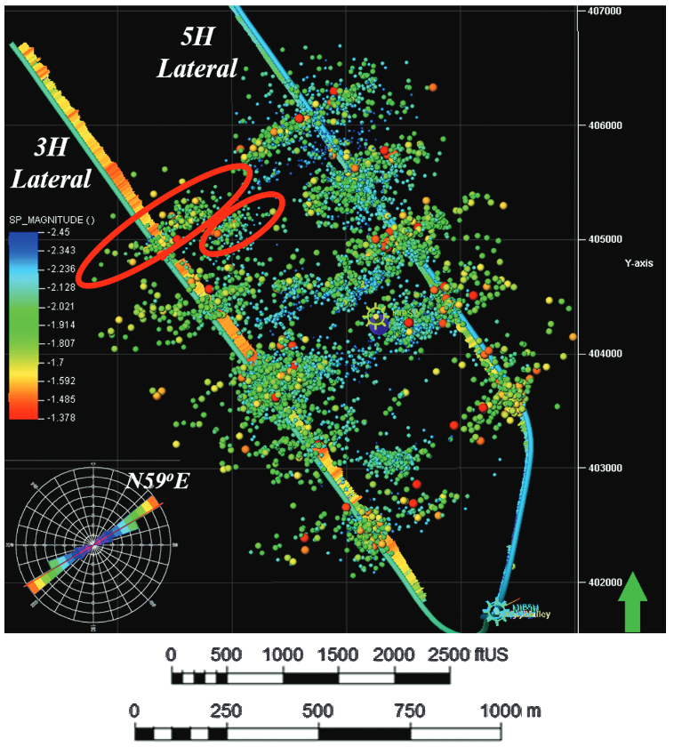
Fig. 131 Shear fracture reactivation in multistage hydraulic fracturing evidenced by microseismic activity - Image from Wilson et al. 2018 - Interpretation

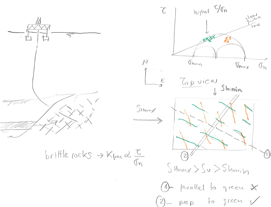
Fig. 132 Example of horizontal wellbore placement in a fractured reservoir. The horizontal wellbore should be ideally perpendicular to critically stressed fractures to take advantage of their high permeability.

The same reasoning applies to large faults. There are faults that may be more easily reactivated due to pore pressure changes because of their orientation with respect to the current state of stress (See subsection \ref{subsec:faultreact}).

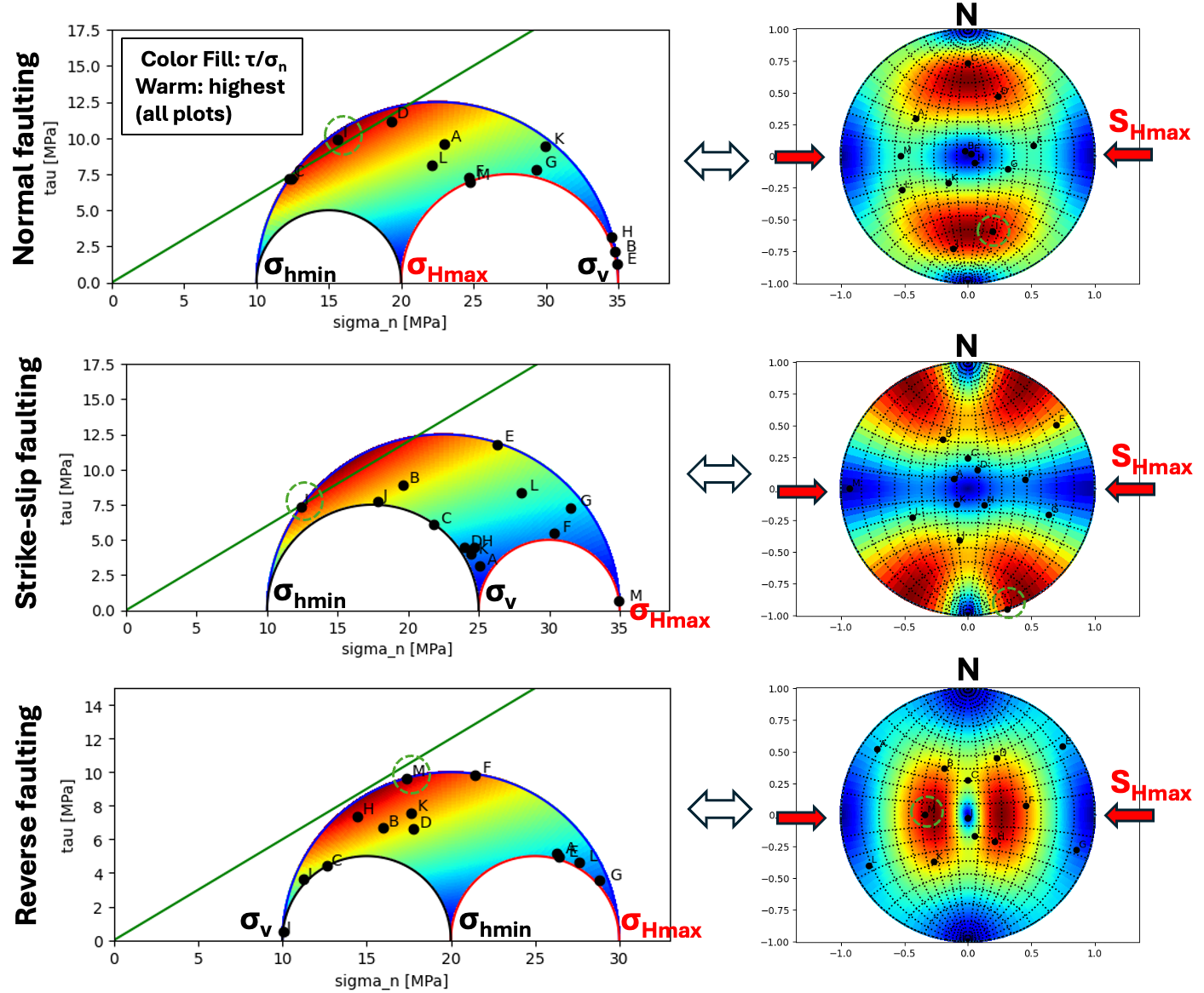
Fig. 133 Examples of fracture plane orientation and corresponding ratio \(\tau / \sigma_n\) and pole location in a stereo-net plot. The orientation of critically stressed fractures varies with faulting regime and principal horizontal stress orientation. This figure was created with the “Tensor method” based on python code initially written by Daniel Barrera (UT Austin BS student, class of 2020).

5.5.2 Determination of horizontal stresses assuming limit equilibrium

Tectonic plates drive movements of the Earth’s crust (Fig. 134). High temperatures and high effective stresses at great depth favor ductile deformation. Low temperatures and low effective stresses in the near-surface favor brittle failure.

Fig. 134 Schematic of a section of the Earth’s crust with brittle failure near surface and ductile deformation at depths greater than \(\sim\) 16 km.

As a result of tectonic movement, there is ubiquitous shear failure and faulting of the Earth’s shallow crust. The frictional strength of faults limits the maximum magnitude of stresses imparted by tectonic strains (Fig. 135). Hence, horizontal stresses are proportional to tectonic strains in the elastic region, but their maximum value is limited by fault strength.

Fig. 135 Schematic of in-situ stress as a function of tectonic strains \(\varepsilon_{tect}\) and failure strength. The frictional strength of faults controls stress once the elastic region is exceeded.

Because faults are cohesion-less, the frictional strength equation is simply:

\[ \sigma_1 = q \: \sigma_3\]

(like sand, zero-intercept in the y-axis) where \(\sigma_1\) is the maximum effective principal stress, \(\sigma_3\) is the minimum effective principal stress, and \(q=[1+\sin(\varphi)]/[1-\sin(\varphi)]\) is the anisotropy factor.

The shear strength of the brittle crust has a direct implication in determining the maximum and minimum values of horizontal stresses for each stress regime once the tectonic strains are surpassed. Frictional equilibrium of the brittle crust implies that minimum and maximum attainable values of horizontal stresses are controlled by shear failure. Hence, for

• normal stress regime (NF): \(\sigma_{hmin}\) cannot be smaller than \(\sigma_{v}/q\), for

• strike-slip stress regime (SS): \(\sigma_{Hmax}\) cannot be greater than \(q \: \sigma_{hmin}\), and for

• reverse stress regime (RF): \(\sigma_{Hmax}\) cannot be greater than \(q \: \sigma_{v}\).

As a result, the assumption of limit frictional equilibrium permits estimating minimum and maximum horizontal stresses if effective stresses \(\sigma_{hmin}\) or \(\sigma_{v}\) are known.

Example 5.13

A given site onshore is known to be subjected to a NF stress regime and hydrostatic pore pressure. Calculate the total horizontal minimum stress \(S_{hmin}\) at a depth of 5,000 ft assuming frictional equilibrium of faults and friction angle \(\varphi = 30^{\circ}\).

SOLUTION

The solution is a lower bound estimation of \(S_{hmin}\) for normal faulting stress regime dictated by frictional equilibrium.

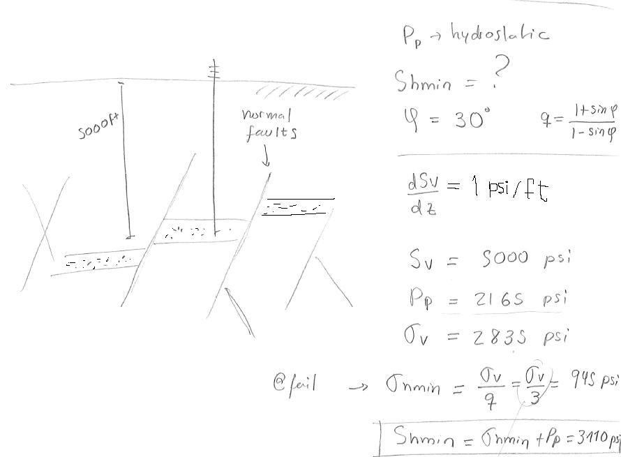
Fig. 136 Solution example 5.13.

\(\: \: \blacksquare\) \newline

Example 5.14

A given site onshore is known to be subjected to a RF stress regime. Hard pressure is detected at 2,000 ft with \(\lambda_p=0.82\). Calculate the total maximum horizontal stress \(S_{Hmax}\) at this depth assuming frictional equilibrium of faults and friction angle \(\varphi = 30^{\circ}\).

SOLUTION

The solution is an upper bound for \(S_{Hmax}\).

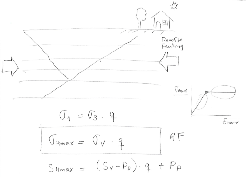
Fig. 137 Solution example 5.14.

Let us assume a lithostatic stress gradient of 1 psi/ft, hence

\( S_v = 1 \text{ psi/ft} \times 2000 \text{ ft} = 2000 \text{ psi} \)

\(S_v\) is the minimum principal since the site is subjected to reverse faulting regime. Given the overpressure parameter, pore pressure is

\( P_p = \lambda_p S_v = 0.82 \times 2000 \text{ psi} = 1640 \text{ psi} \)

and effective vertical stress is

\( \sigma_v = S_v - P_p = 2000 \text{ psi} - 1640 \text{ psi} = 360 \text{ psi} \)

Finally, the maximum effective horizontal stress depends on the vertical effective stress (reverse faulting regime), so that

\( \sigma_{Hmax} = q \: \sigma_v = \frac{1+\sin 30^{\circ}}{1-\sin 30^{\circ}} 360 \text{ psi} = 1080 \text{ psi} \) and therefore

\( S_{Hmax} = \sigma_{Hmax} + P_p = 1080 \text{ psi} + 1640 \text{ psi} = 2720 \text{ psi} \: \: \blacksquare \)

The bounding limits of minimum and maximum horizontal stress for a given vertical stress and pore pressure can be plotted through Zoback’s (effective) stress polygon (Fig. 138). The colored lines represent the bounds for normal faulting stress regime (NF), strike-slip faulting stress regime (SS), and reverse faulting stress regime (RF).

Fig. 138 The limits of horizontal stresses based on frictional equilibrium can be conveniently plotted in a “stress polygon” plot.

For example, the state of stress for a place with a stress regime that fluctuates from NF to SS with depth would plot at the intersection of NF and SS lines in the stress polygon (Fig. 139).

Fig. 139 Application example of the stress polygon. This particular place exhibits a hybrid stress regime NF and SS depending on depth and likely rock lithology.

5.5.3 Determination of stress regime and horizontal stress direction from fault orientation

Mapping of faults and fractures in the subsurface helps interpret the state of stress that caused such fractures. In some cases the state of stress that caused such faults may be still acting today. The example in Fig. 140 shows an example of strike-slip conjugate faults. The maximum horizontal stress that caused these shear faults was aligned with the bisectrix of the two fault strikes, about E10\(^{\circ}\)S.

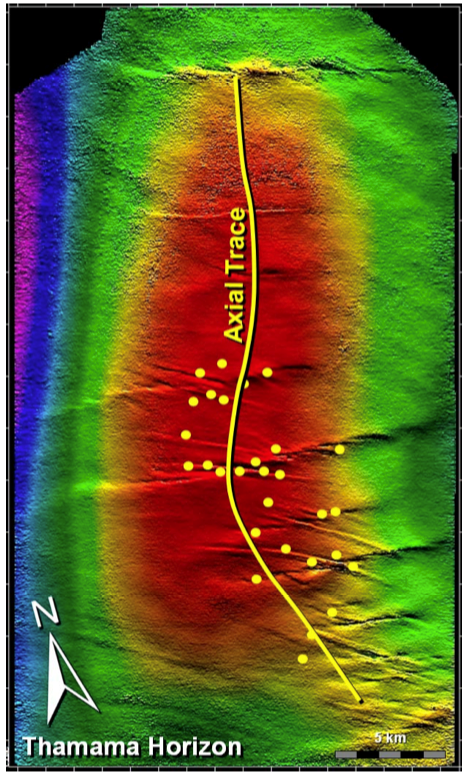
Fig. 140 Seismic image of the top of an anticline structure (red: shallower, blue: deeper, TOP VIEW). The discontinuities in the seismic image are strike-slip faults. Image from IPTC-10646-MS.

5.5.4 Fault reactivation

Depletion and injection of fluids in the subsurface cause changes in pore pressure and therefore on effective stresses. Fluid injection such as in hydraulic fracturing, water-flooding, and waste-water disposal can reach adjacent faults (if any) and decrease the effective normal stress \(\sigma_n = S_n - P_p\) acting on faults. In hydraulic fracturing, the injection of fluids is temporary and limited to the fracture completion size. In water-flooding, pressure build-up is limited by the producer wells. In waste-water injection (including salt-water disposal SWD), the pressure build-up is controlled by the aquifer size, compressibility and compartmentalization.

Fig. 141 Fault reactivation. Injection of fluids changes the pore pressure and lowers effective normal stress on faults increasing \(\tau/\sigma_n\).

The change of stresses produced by increases of pore pressure assuming constant total vertical stress and negligible poroelastic effects is

\[\begin{split} \left\lbrace \begin{array}{l} \Delta \sigma_v = - \Delta P_p \\ \Delta \sigma_{hmin} \leq - \Delta P_p \\ \end{array} \right.\end{split}\]

The result is a shift of the Mohr circle to the left, closer to the shear failure or ``reactivation’’ line. The magnitude of change of pore pressure needed to reactivate a fault is (at least) equal to the horizontal distance between the point of the Mohr-circle of such fault and the failure line. Hence, a critically oriented fracture needs the lowest \(\Delta P_p\) to reactivate.

The reactivation of faults may result in induced seismicity. The imparted change of fault permeability depends on the fault filling, known as fault gouge. Both, induced seismicity and change in fault permeability depend on the failure properties of the fault gouge. Brittle failure results in high energy release through induced seismicity and increases of fault permeability, while ductile failure results in low energy release through seismicity and decreases or minor increases of permeability. An undesired consequence of fault reactivation is the loss of hydrocarbon trapping ability at fault structural traps (Video example from Frade Field).

Induced seismicity triggered by subsurface fluid injection has become a major concern and sometimes a show-stopper in the energy industry. Salt-water disposal from oil and gas activity has caused “unseen” earthquakes in modern history in Oklahoma and Texas. Fig. 142 shows images relating salt-water disposal volumes, ground elevation change (discussed Chapter 8), and induced seismicity in the Delaware Basin near the city of Pecos. The field evidence indicated that seismicity and ground elevation change are caused by reactivation of faults due to subsurface fluid withdrawal (oil and gas) and injection (produced and back-flow water).
Other energy applications are not excempt of geomecahnical consequences. The Pohang earthquake is a well known example of fault reactivation risk induced by enhanced geothermal activities. Fig. 143 shows an example of induced seismicity with magnitude \(M<2\) in the Richter scale due to injection of carbon dioxide in the Mount Simon Sandstone. The seismicity originates mostly from reactivation of faults below the reservoir formation in basement formations. The regional stress regime alternates between strike-slip and reverse (See fig:USGSstressmap).

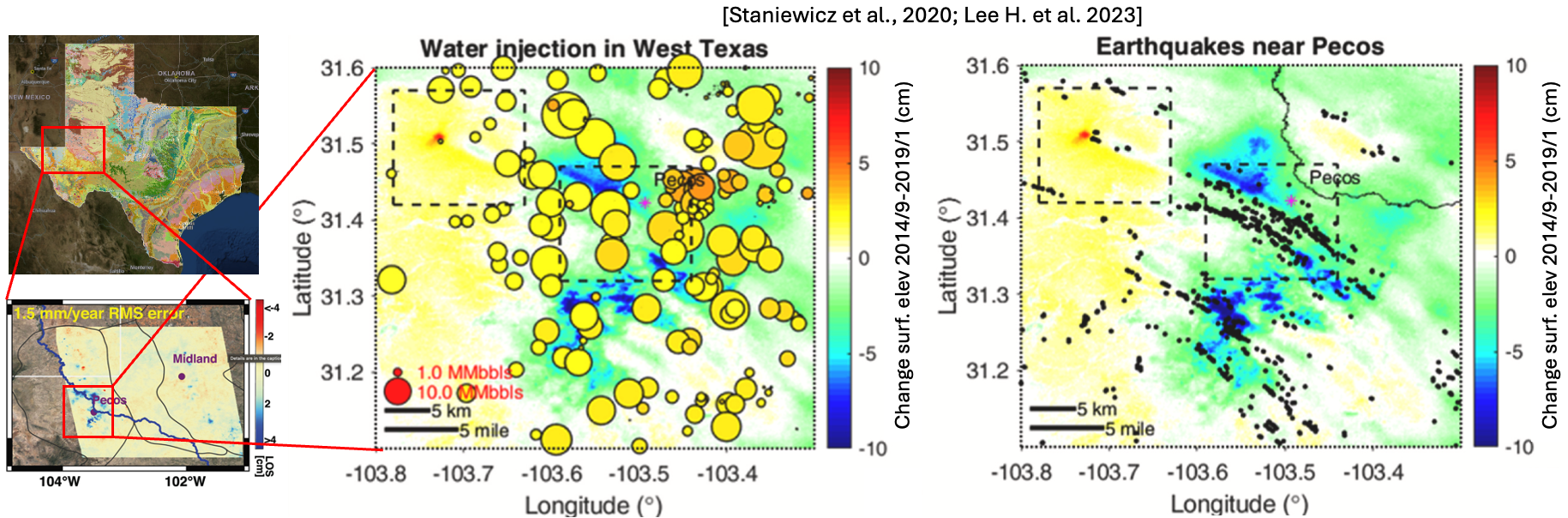
Fig. 142 Fault reactivation and induced seismicity linked to saltwater disposal in the Delaware Basin, Texas (Image credit: 1 and 2).

Fig. 143 Fault reactivation observed through microseismicity due to CO\(_2\) injection in a sandstone formation Bauer et al, 2016 - IJGGC. Notice the alignment of events that likely reveals fault strike. Significant microseismicity occurs as far as 0.6 miles away from the injector.

5.6 Problems

1. For the following faults: (i) draw the corresponding points in a stereonet (lower hemisphere projection) map, and (ii) convert strike from quadrant to azimuth convention. Use this web app by Visible Geology and this mobile app by Prof. Allmendinger only to verify your answers.

   • N55\(^{\circ}\)E, 45\(^{\circ}\)SE

   • E20\(^{\circ}\)S, 60\(^{\circ}\)NE

   • N20\(^{\circ}\)W, 25\(^{\circ}\)SW

   • S10\(^{\circ}\)W, 60\(^{\circ}\)NW

2. Find out the ideal orientations of (a) a hydraulic fracture and (b) shear fractures, all created in a site subjected to stresses \(S_v < S_{hmin} < S_{Hmax}\) where \(S_{Hmax}\) strikes E-W, \(\mu =\) 0.8, and \(S_v\) is a principal stress.

3. Find out the ideal orientations of (a) a hydraulic fracture and (b) shear fractures, all created in a site subjected to stresses \(S_{hmin} < S_{v} < S_{Hmax}\) where \(S_{Hmax}\) strikes W20\(^{\circ}\)N, \(\mu=0.5\), and \(S_v\) is a principal stress..

4. Find out the state of stress (regime and direction of stresses) that caused the faults mapped in the following stereonets:

Fig. 144 Problem 4.

5. In a given reservoir under study, stresses are \(S_{hmin}=\) 40 MPa, \(S_{Hmax}=60\) MPa, \(S_v=45\) MPa, \(P_p= 20\) MPa, and \(S_{hmin}\) acts E-W. For each of the faults below, calculate (using the 3D Mohr circle method if possible) the normal and shear stress on the plane of the fault and then determine if the fault is prone to slip assuming \(\mu = 0.6\).

   1. Fault with strike north-south, dip 65\(^{\circ}\) to the east

   2. Fault with strike east-west, dip 35\(^{\circ}\) to the north

   3. Fault with strike 060\(^{\circ}\), dip 90\(^{\circ}\)

   4. Fault with strike 030\(^{\circ}\), dip 25\(^{\circ}\)

6. (Optional) Write a Matlab/Python code that can obtain (\(S_n\), \(\sigma_n\), \(\tau_d\), \(\tau_s\)) on an arbitrary fault with orientation \((strike, dip)\) for a given state of stress \((\underset{=}{S}{}_P, \alpha, \beta, \gamma)\).

   1. Verify with solved problems in this chapter

   2. Apply to solve all cases in Problem 5

   3. Apply code to solve stress on 100 fractures randomly oriented with the stresses of Problem 5. Plot all results the respective 3D Mohr circle. A nearby injection wellbore will perform water flooding. What is the additional pore pressure needed to start reactivating faults?

   Hint: Matlab function ‘rand’ can be used for creating an array of random values; \(r = a + (b-a)*rand(N,1)\) creates an array \(r\) (Nx1) of values in interval \([a,b]\)

7. Let us compare reservoirs with normal and reverse faulting regimes (onshore). For both regimes, plot the limits of \(S_1\) and \(S_3\) versus depth from 0 to 5 km assuming lithostatic gradient equal to 23 MPa/km, hydrostatic pore pressure equal to 10 MPa/km, and a state of stress limited by frictional strength of faults. Assume sliding friction coefficient is \(\mu =\) 0.6. For both regimes, how does changing \(\mu\) from 0.6 to 1.0 change the maximum possible differential stress \(S_1-S_3\) at a fixed depth of \(z=5\) km?

8. A given site offshore (sea floor at 500 ft) is subjected to a Normal Faulting stress regime. Over-pressure exists and at 2,000 ft (TVDSS: True Vertical Depth Sub-Sea) overpressure is \(\lambda_p =\) 0.78. Calculate the total minimum horizontal stress \(S_{hmin}\) at this depth (2,000 ft TVDSS) assuming frictional equilibrium of faults and friction angle 30\(^{\circ}\). Draw the corresponding 2D Mohr circle with a solid line and draw an additional 2D Mohr circle with a dashed line assuming hydrostatic pressure. (Assume typical water and lithostatic gradients)

9. The following figure shows major faults in the Eagle Ford region [EIA, 2014 - Updates to the EIA Eagle Ford Play Maps].

   1. Looking at the normal faults in the Frio, Atascosa, and Wilson counties, what would be the expected direction of the minimum horizontal stress \(S_{hmin}\) in this area?

   2. Visit the GIS application of the railroad commission of Texas. Zoom into the South-East of the Frio county until you see well trajectories. The horizontal wells are expected to be drilled in the direction of the least principal stress. Does this direction of \(S_{hmin}\) coincide with the direction expected from fault orientation? Justify.

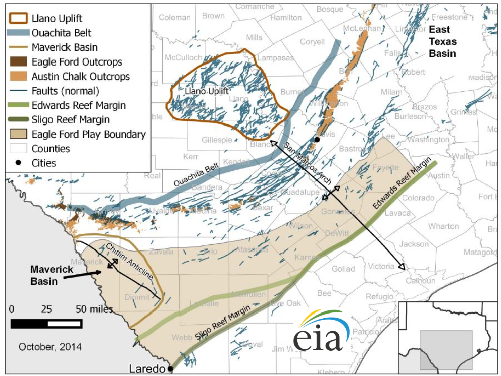
Fig. 145 Problem 5.9.

5.7 Coding support for solving problems

You may use the python code available in the following link at Google Colab: Ch. 5 - Stresses on Faults and Fractures. I suggest you use it as “inspiration” and learning, but write your own. Make sure to acknowledge any copying and pasting.

5.8 Further reading and references

• Zoback, M.D., 2010. Reservoir geomechanics. Cambridge University Press. (Chapters 5 and 9)