4. Inelasticity

4.1 Examples of inelasticity in the subsurface

Figure 4.1: Examples of inelasticity in subsurface applications.

4.2 The yield surface

Figure 4.2: General equation of the yield surface.

4.2.1 Tresca

Figure 4.3: Tresca's yield surface.

4.2.2 Von Mises

Figure 4.4: von Mises' yield surface.

4.2.3 Mohr-Coulomb and Drucker-Prager

Figure 4.5: The friction coefficient.

Figure 4.6: Intergranular friction, failure angle and maximum stress anisotropy.

Figure 4.7: Mohr Coulomb and Drucker Prager in various stress spaces.

Figure 4.8: Measurement of shear strength.

4.2.4 Lade

Figure 4.9: The modified Lade criterion.

4.2.5 Mogi

TBD

4.3 Plastic strains

Figure 4.10: Determination of plastic strains.

Figure 4.11: Determination of plastic strains with Mohr-Coulomb associated flow rule.

Figure 4.12: Determination of plastic strains with Mohr-Coulomb associated flow rule (continued).

Figure 4.13: Non-associated flow rule - general concepts.

4.4 WP7: Rock Failure and Application to Wellbore Stability

4.4.1 Exercise 1: Determination of shear and tensile strength

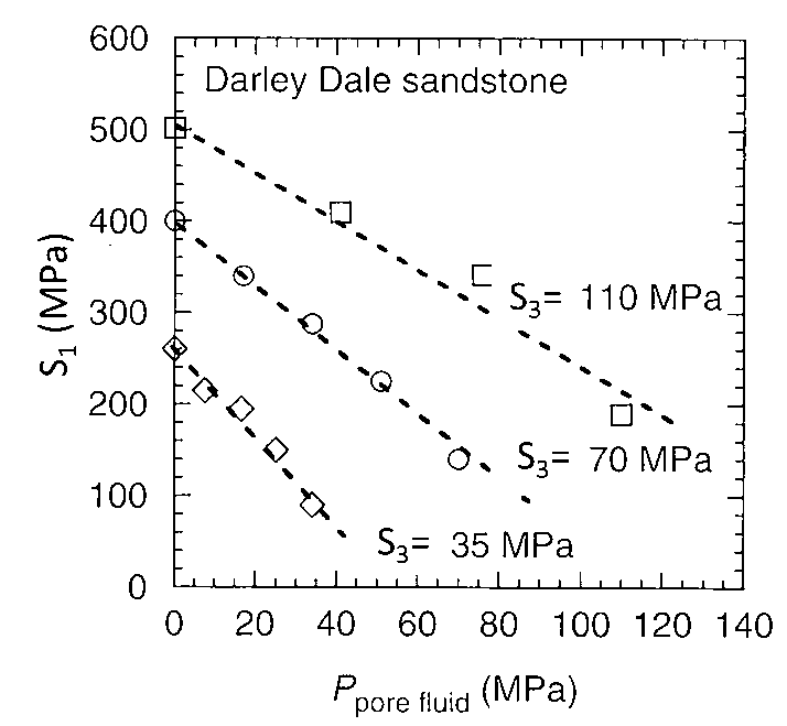
The following data set has experimental data of shear strength for the Darley Dale Sandstone measured in an axisymmetric triaxial cell.

Figure 4.14: Peak stress measured from triaxial tests (image source: Jaeger et al. 2007 - FRM 4th Ed).

where $S_1$ is the maximum total principal stress, $S_3$ is the minimum total principal stress, and $P_{pore \: fluid}$ is the pore pressure in the rock.

1. Determine the best fitting parameters of a Coulomb criterion: $\sigma_1 = UCS + q \sigma_3$.
2. Determine the corresponding values of cohesive strength $S_0$ and friction angle $\varphi$ from point (1) and draw the shear failure line together with Mohr circles at failure.
3. Determine the corresponding fitting parameters for a Drucker-Prager criterion and plot experimental data in a $I_1$ v.s. $(J_2)^{1/2}$ space.
4. Compute the corresponding tensile strength assuming a reasonable ratio of unconfined compression strength to tensile strength (browse Jaeger’s book).

4.4.2 Exercise 2: Shear and tensile failure in vertical and deviated wellbores

For this assignment you have to be able to calculate principal stresses on the wall of a wellbore at an arbitrary deviation and azimuth (See Chapter 6 of my notes “Wellbore stability” (https://dnicolasespinoza.github.io/) and Zoback's book Ch. 8).

Develop a script to compute and illustrate graphically (lower hemisphere projection):

1. The likelihood of tensile fractures considering wellbore mud pressure is equal to pore pressure in the formation $P_W = P_p$ and a simple tensile strength criterion (independent of intermediate and maximum principal stresses), i.e., required $T_s$.
2. The likelihood of breakouts considering wellbore mud pressure is equal to pore pressure in the formation $P_W = P_p$ and a simple unconfined compression strength criterion, i.e., required $UCS$.
3. The wellbore breakout angle $w_{BO}$ considering a Mohr-Coulomb shear failure criterion and the properties of the Darley Dale Sandstone from Exercise 1.
4. The wellbore breakout angle $w_{BO}$ considering a linear $I_1$ v.s. $(J_2)^{1/2}$ shear failure criterion and the properties of the Darley Dale Sandstone from Exercise 1.
5. The wellbore breakout angle $w_{BO}$ considering a Modified Lade shear failure criterion (Zoback's book, p. 100) and the properties of the Darley Dale Sandstone from point 1.

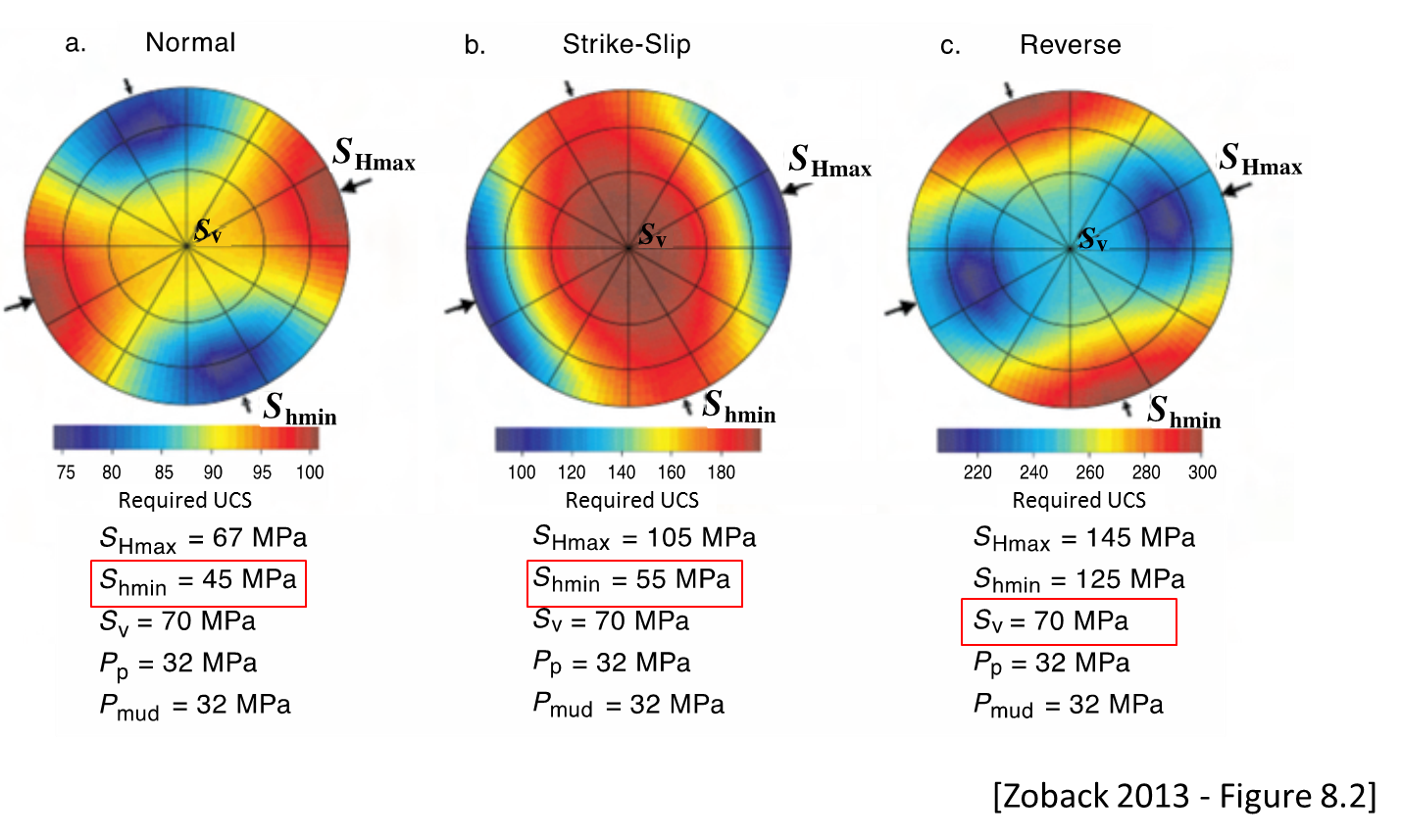
Limit your wellbore breakout angle plots to $0^{\circ} < w_{BO} < 60^{\circ}$ because predictions with linear elasticity over $w_{BO} > 60^{\circ}$ are likely highly inaccurate. Test your script with the three examples given in Zobacks's book in Figures 8.2 and 10.4 (normal faulting, strike-slip faulting, and reverse faulting). When computing breakouts assume $P_W$ = 32 MPa (NF), $P_W$ = 40 MPa (SSF), and $P_W$ = 52 MPa (RF). Use a Poisson ratio of 0.25 for stress calculations.

Figure 4.15: Wellbore stability results plotted as lower hemisphere projections (image source: Zoback 2013 - RG). Note: $P_{mud} = P_W$ in the figure above.

4.5 Critical state soil mechanics

Figure 4.16: Cam-clay - introduction.

4.5.1 Yield surface and the critical state line

Figure 4.17: The yield surface and effect of confinement for strain hardening and strain softening behavior.

Figure 4.18: Slope of the critical state line.

Figure 4.19: The yield surface.

Figure 4.20: Hardening as a function of volumetric plastic strain.

Figure 4.21: Void ratio.

Figure 4.22: Yield surface including void ratio.

4.5.2 Calculation of elastic and plastic strains

Figure 4.23: Partition of elastic and plastic strain.

Figure 4.24: The oedometer setup to measure elastic and plastic strain.

Figure 4.25: Elastic and plastic non-linear volumetric strain.

Figure 4.26: Elastic stiffnes matrix.

Figure 4.27: Plastic strains from associated flow rule.

Figure 4.28: Plastic stiffnes matrix.

Figure 4.29: Strain localization as a result of strain softening.

4.6 Brittle to ductile transition

Figure 4.30: Example of brittle to ductile transition.

Figure 4.31: Effects of mean effective stress and temperature on brittle to ductile transition.

Figure 4.32: Other influencing factors on brittle to ductile transition.

4.7 Special cases for changes in the yield surface

Figure 4.33: Kinematic hardening and chemo-plasticity.

4.8 Visco-elasticity and Visco-plasticity

Figure 4.34: Manifestations of time-dependent deformation.

4.9 WP8: Soft Sediment Constitutive Models

4.9.1 Exercise 1: Compressibility of mudrocks

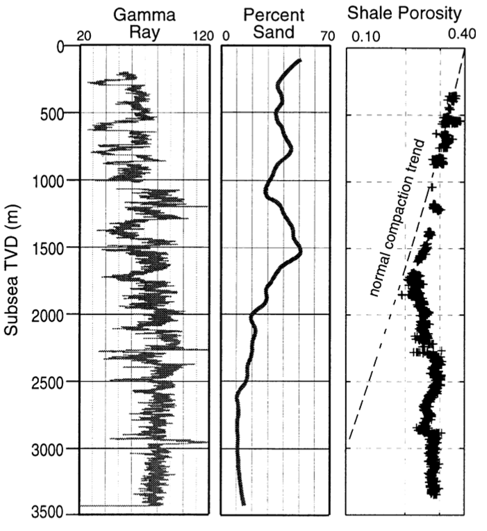
The following data set contains well-logging measurements of porosity of a mudrock as a function of depth (Eugene Island – offshore Louisiana):

Figure 4.35: Example of shale dis-equilibrium compaction evidenced by porosity deviation from the normal compaction trend (image source: Gordon and Flemings, 1998 https://doi.org/10.1046/j.1365-2117.1998.00052.x). Note about subplot 3: The x-axis “Shale Porosity” goes from 0.1 to 0.4 in logarithmic scale.

1. Compute and plot pore pressure assuming a hypothetical hydrostatic pore pressure gradient $dP_p/dz$ = 0.465 psi/ft.
2. Compute and plot total vertical stress assuming $dS_v/dz$ = 0.950 psi/ft and pick the seafloor from the shallowest data point in “percent sand” plot.
3. Digitize shale porosity data (at least 20 equally spaced points) and fit an equation of porosity as a function of vertical effective stress from depth 400 m to 1800 m assuming hydrostatic pore pressure and models:
   Exponential on porosity: $\phi = \phi_0 \exp \left(-\beta\sigma_v \right)$
   Logarithmic on void ratio: $e = e_0 - C_c \ln \left(\frac{\sigma_v}{1 \text{ MPa}} \right)$
   Show the porosity-effective vertical stress and void ratio-effective vertical stress plots.
4. Calculate and plot actual pore pressure between the interval 1800 m to 3400 m assuming porosity is a function of vertical effective stress with the models calculated in point 3.
5. Calculate and plot overpressure parameter $\lambda_p$ as a function of depth.
6. Summarize all results with plots of
   (Left) Porosity (model and data) in log scale as a function of depth (y-axis)
   (Middle) $S_v$ and actual $P_p$ as a function of depth (y-axis)
   (Right) Overpressure parameter as a function of depth (y-axis)

4.9.2 Exercise 2: Cam-clay model

Write a script that simulates a (axisymmetric) triaxial loading test ( $dq=3dp^\prime$) for a mudrock with the following properties:

• Elastic shear modulus, $G$ = 1 MPa;
• Pre-consolidation stress, $p'_o$ = 250 [kPa]
• Friction angle at critical state, $\phi_{CS} = 24^{\circ}$
• Loading compressibility, $\lambda$ = 0.25;
• Unloading compressibility, $\kappa$ = 0.05;
• Initial void ratio, $e_o$ = 1.15;

The initial state of stress is $p'$= 200 kPa; $q$ = 0 kPa. Load the sample until the critical state.

1. Plot the stress path $q$ versus $p'$. Plot the initial yield surface and the final yield surface. Is there hardening or softening?
2. Plot $q$ as a function of $\varepsilon_q$. Why does it approximate an asymptotic value?
3. Plot void ratio $e$ as a function of $p'$ (with $p'$ in logarithmic scale). Why is there a clear change of slope?
4. EXTRA: Repeat the exercise from the initial condition for a uniaxial-strain stress path approximated by $dq=0.9 \: dp^\prime$, up to $p^\prime = 400$ kPa). Plot the stress path $q$ versus $p'$ and void ratio $e$ as a function of $p'$ (with $p'$ in logarithmic scale). Compare the uniaxial-strain stress-path with the triaxial deviatoric loading stress path.

Equations:
Incremental elastic deformations: $d\varepsilon_{p^\prime}^e = \frac{\kappa}{\upsilon} \frac{dp^\prime}{p^\prime}; \: d\varepsilon_q^e = \frac{dq}{3G}$
Incremental plastic deformation: $\left[ \begin{matrix} d\varepsilon_{p^\prime}^p \\ d\varepsilon_q^p\\ \end{... ...trix} \right] \left[ \begin{matrix} dp^\prime \\ dq \\ \end{matrix}\right]$

where $\upsilon=1+e$ is the specific volume, $\eta=q/p'$, and $de= -\upsilon d\varepsilon_p$.

The incremental change of the yield surface is: $dp_o^\prime = d\varepsilon_{p^\prime}^p \frac{\upsilon}{\lambda-\kappa} p_o^\prime$.

4.10 Suggested Reading

• Deviated wellbores in anisotropic rock: https://doi.org/10.1016/j.ijrmms.2018.10.033
• Soils and Waves: Particulate Materials Behavior, Characterization and Process Monitoring, https://www.wiley.com/en-ie/Soils+and+Waves:+Particulate+Materials+Behavior,+Characterization+and+Process+Monitoring-p-9780471490586.
• FLAC Manual, https://docs.itascacg.com/flac3d700/common/models/camclay/doc/modelcamclay.html