5.9 WP8: Soft Sediment Constitutive Models

5.9.1 Exercise 1: Compressibility of mudrocks

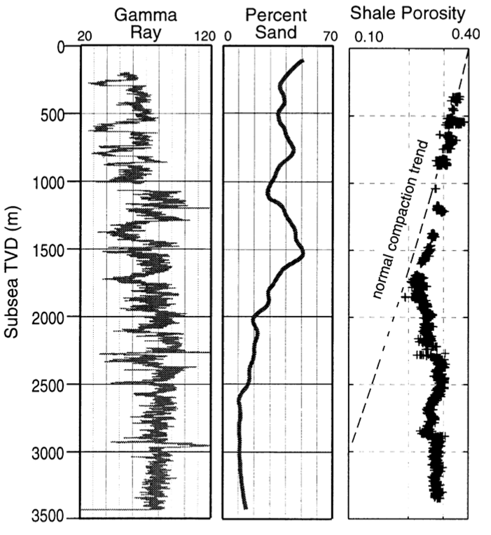
The following data set contains well-logging measurements of porosity of a mudrock as a function of depth (Eugene Island – offshore Louisiana):

**Figure 5.3:** Example of shale dis-equilibrium compaction evidenced by porosity deviation from the normal compaction trend (image source: Gordon and Flemings, 1998 `https://doi.org/10.1046/j.1365-2117.1998.00052.x`). Note about subplot 3: The x-axis “Shale Porosity” goes from 0.1 to 0.4 in logarithmic scale.

a.: Compute and plot pore pressure assuming a hypothetical hydrostatic pore pressure gradient = 0.465 psi/ft.
b.: Compute and plot total vertical stress assuming = 0.950 psi/ft and pick the seafloor from the shallowest data point in “percent sand” plot.
c.: Digitize shale porosity data (at least 20 equally spaced points) and fit an equation of porosity as a function of vertical effective stress from depth 400 m to 1800 m assuming hydrostatic pore pressure and models:
Exponential on porosity: $\phi = \phi_0 \exp \left(-\beta\sigma_v \right)$
Logarithmic on void ratio: $e = e_0 - C_c \ln \left(\frac{\sigma_v}{1 \text{ MPa}} \right)$
Show the porosity-effective vertical stress and void ratio-effective vertical stress plots.
d.: Calculate and plot actual pore pressure between the interval 1800 m to 3400 m assuming porosity is a function of vertical effective stress with the models calculated in point 3.
e.: Calculate and plot overpressure parameter $\lambda_p$ as a function of depth.
f.: Summarize all results with plots of
(Left) Porosity (model and data) in log scale as a function of depth (y-axis)
(Middle) and actual as a function of depth (y-axis)
(Right) Overpressure parameter as a function of depth (y-axis)

5.9.2 Exercise 2: Cam-clay model

Write a script that simulates a (axisymmetric) triaxial loading test ( $dq=3dp^\prime$ ) for a mudrock with the following properties:

Elastic shear modulus, = 1 MPa;
Pre-consolidation stress, = 250 [kPa]
Friction angle at critical state, $\phi_{CS} = 24^{\circ}$
Loading compressibility, $\lambda$ = 0.25;
Unloading compressibility, $\kappa$ = 0.05;
Initial void ratio, = 1.15;

The initial state of stress is $p'$ = 200 kPa; $q$ = 0 kPa. Load the sample until the critical state.

a.: Plot the stress path versus . Plot the initial yield surface and the final yield surface. Is there hardening or softening?
b.: Plot as a function of $\varepsilon_q$ . Why does it approximate an asymptotic value?
c.: Plot void ratio as a function of (with in logarithmic scale). Why is there a clear change of slope?
d.: EXTRA: Repeat the exercise from the initial condition for a uniaxial-strain stress path approximated by $dq=0.9 \: dp^\prime$ , up to $p^\prime = 400$ kPa). Plot the stress path versus and void ratio as a function of (with in logarithmic scale). Compare the uniaxial-strain stress-path with the triaxial deviatoric loading stress path.

Equations:
Incremental elastic deformations: $d\varepsilon_{p^\prime}^e = \frac{\kappa}{\upsilon} \frac{dp^\prime}{p^\prime}; \: d\varepsilon_q^e = \frac{dq}{3G}$
Incremental plastic deformation: $\left[ \begin{matrix} d\varepsilon_{p^\prime}^p \\ d\varepsilon_q^p\\ \end{... ...trix} \right] \left[ \begin{matrix} dp^\prime \\ dq \\ \end{matrix}\right]$

where $\upsilon=1+e$ is the specific volume, $\eta=q/p'$ , and $de= -\upsilon d\varepsilon_p$ .

The incremental change of the yield surface is: $dp_o^\prime = d\varepsilon_{p^\prime}^p \frac{\upsilon}{\lambda-\kappa} p_o^\prime$ .