2.7 WP4: Solution of Navier's Equation for the Stress Field

2.7.1 Exercise 1: Stresses around a wellbore

Consider a 2D problem of a circular cavity subjected to far field effective stresses $\sigma_{xx}$ = 12 MPa and $\sigma_{yy}$ = 3 MPa. The diameter of the cavity is 0.2 m. Rock properties: $E$ = 10 GPa, $\nu$ = 0.20, unconfined compression strength $UCS$ = 30 MPa, tensile strength $T_s$ = 2 MPa.

a.

Using Kirsch equations compute (and plot) $\sigma_{rr}$, $\sigma_{\theta\theta}$ and $\sigma_{r\theta}$ for a domain $x$ = [-1m, +1m], and $y$ = [-1m, +1m]. You may define a polar grid for $(r,\theta)$. How far does the presence of the wellbore influence stresses?

b.

Using Kirsch equations compute (and plot) stresses in a line ($x$ = [0.1m, 1m], $y$ = 0 m) and ($x$ = 0 m, $y$ = [0.1 m, 1 m]). Equations in Ch. 6.2 (https://dnicolasespinoza.github.io/)

c.

Using Kirsch equations compute (and plot) $\sigma_{rr}$ and $\sigma_{\theta\theta}$ for $r$ = 0.1 m. Is there any section of the rock in shear or tensile failure? Where?

d.

Use FreeFEM++ (http://www3.freefem.org/) or FEniCS (https://fenicsproject.org/) to solve the same problem ( $\sigma_{xx}$, $\sigma_{yy}$ and $\sigma_{xy}$) assuming a domain size 2 m by 2 m. Compute $\sigma_{xx}$ and $\sigma_{yy}$ for the same lines as in point (b), and compare with Kirsch's analytical solution. Repeat the process for a domain size 0.5 m by 0.5 m. Are there any differences? Why?

e.

Plot the displacement field.

f.

EXTRA: compute principal stresses within FreeFEM++ and plot $\sigma_{rr}$ and $\sigma_{\theta\theta}$.

Hint: An example code for 2D elasticity in FreeFEM++ and the corresponding explanation are available at https://github.com/dnicolasespinoza/GeomechanicsJupyter/: Kirsch_Shovkun.edp and FreeFEM_Tutorial_Shovkun.pdf. You can also try FreeFEM++ online here: https://freefem.org/tryit.

2.7.2 Exercise 2: Stresses around a planar fracture

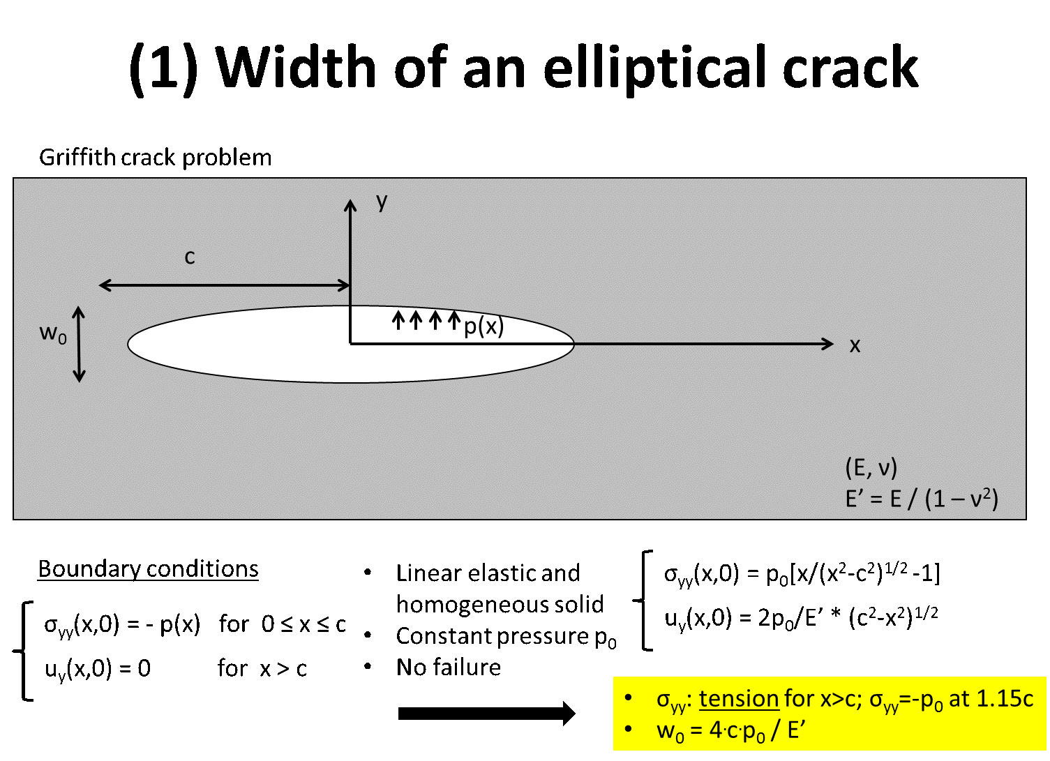
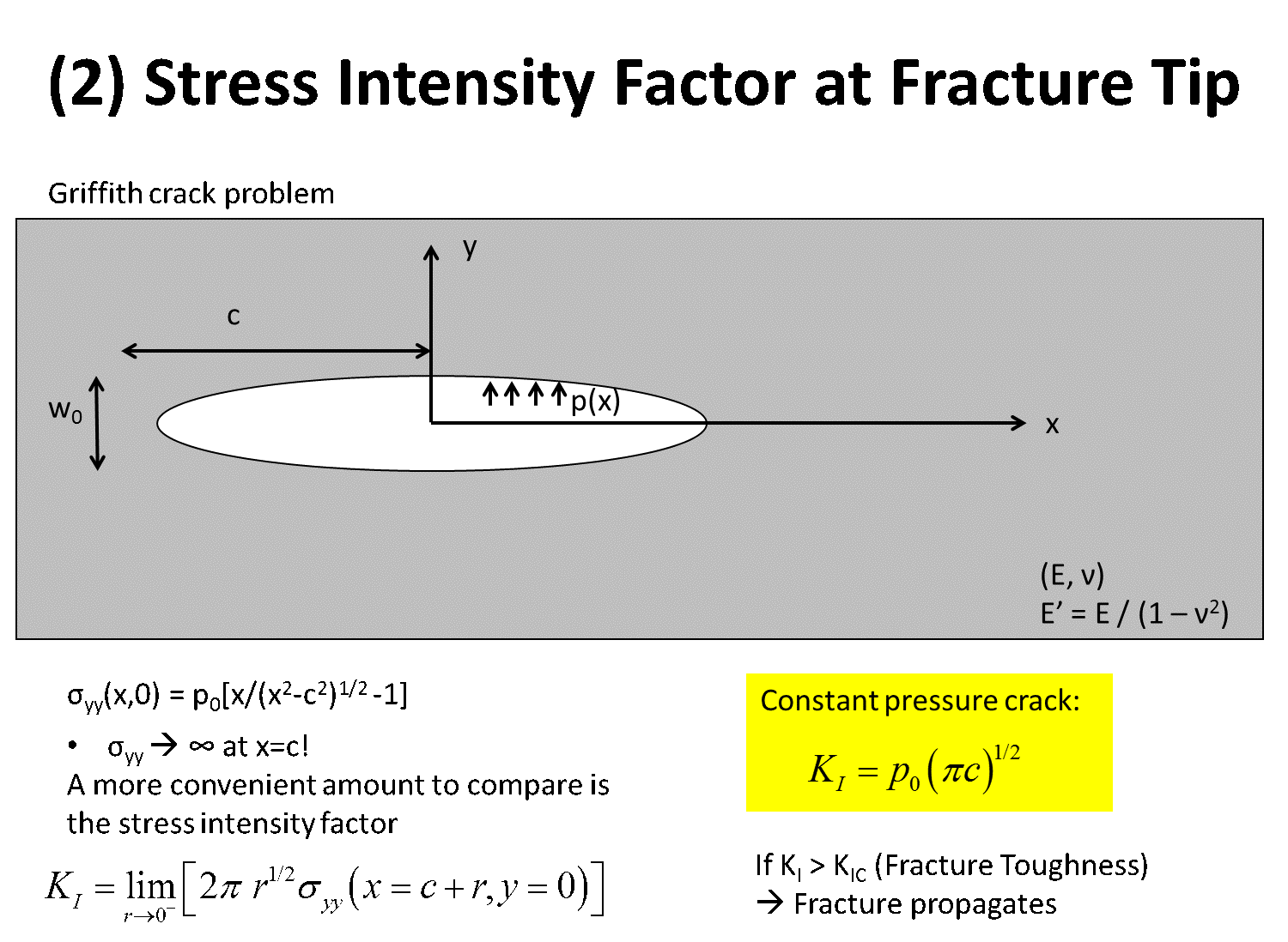
Consider a 2D problem of an elliptical fracture (half-length $c$ = 10 m). Solve the problem using just half of the domain. Set the fracture along the left boundary of a domain: $x$ = [0 m, 100 m] and $y$ = [-50 m, 50 m], with fracture center at $(x,y)=$ (0,0) m. This boundary will have a pressure boundary condition. All other boundaries will have zero displacement. Rock properties: $E$ = 30 GPa, $\nu$ = 0.20.

Figure 2.2: Planar fracture model.

a.

Use FreeFEM++ (http://www3.freefem.org/) or FEniCS (https://fenicsproject.org/) to solve for $\sigma_{xx}$, $\sigma_{yy}$ and $\sigma_{xy}$ imposing a fracture pressure $p$ = 10 MPa. Plot results.

b.

Export and plot stress perpendicular to the fracture direction $\sigma_{xx}$ at the middle of the fracture (L1 = ($x$ = [0, 100 m], $y$ = 0 m), Figure 2.2). How far does the influence of the fracture extend?

c.

Plot $x$-displacements at the face of the fracture. Compare with analytical equation. Equations in Ch. 7.3.2 (https://dnicolasespinoza.github.io/).

d.

Plot $\sigma_{xx}$ along fracture length and beyond fracture tips (line L2 = ($x$ = 0 m, $y=$ [-50, 50]) m, Figure 2.2) and compare with analytical Griffith solution.

e.

EXTRA: compare FreeFEM++ solution to analytical solution by Sneddon and Elliot, 1946. (Eq. 20 in https://doi.org/10.1016/j.fuel.2017.01.057).

Figure 2.3: Fracture width and stress beyond tip.

Figure 2.4: Stress intensity factor.